Users' Manual - IRIT
A Solid Modeling Program
(C) Copyright 1989-2023 Gershon Elber
| EMail: | 
|
|---|---|
| Join IRIT mailing list: | 
|
| Mailing list: | 
|
| Bug reports: | 
|
| WWW Page: | http://gershon.cs.technion.ac.il/irit |
This manual is for IRIT Ver. 13
Copyright (C) 1989-2023 Gershon Elber
EMail: gershon@cs.technion.ac.il
Join IRIT mailing list: gershon@cs.technion.ac.il
Mailing list: irit-mail@cs.technion.ac.il
Bug reports: irit-bugs@cs.technion.ac.il
WWW Page: http://gershon.cs.technion.ac.il/irit
Introduction
IRIT is a solid modeler developed for educational purposes. Although small, it is now powerful enough to create quite complex scenes.IRIT started as a polygonal solid modeler and was originally developed on an IBM PC under MSDOS. Version 2.0 was also ported to X11 and version 3.0 to SGI 4D systems. Version 3.0 also includes quite a few free form curves and surfaces tools. See the UPDATE.NEW file for more detailed update information. In Version 4.0, the display devices were enhanced, freeform curves and surfaces are more extensively supported, functions can be defined, and numerous improvement and optimizations are added.
Copyrights
BECAUSE IRIT AND ITS SUPPORTING TOOLS AS DOCUMENTED IN THIS DOCUMENT ARE LICENSED FREE OF CHARGE (FOR NON COMMERCIAL USE), I PROVIDE ABSOLUTELY NO WARRANTY, TO THE EXTENT PERMITTED BY APPLICABLE STATE LAW. EXCEPT WHEN OTHERWISE STATED IN WRITING, I GERSHON ELBER PROVIDE THE IRIT PROGRAM AND ITS SUPPORTING TOOLS "AS IS" WITHOUT WARRANTY OF ANY KIND, EITHER EXPRESSED OR IMPLIED, INCLUDING, BUT NOT LIMITED TO, THE IMPLIED WARRANTIES OF MERCHANTABILITY AND FITNESS FOR A PARTICULAR PURPOSE. THE ENTIRE RISK AS TO THE QUALITY AND PERFORMANCE OF THESE PROGRAMS IS WITH YOU. SHOULD THE IRIT PROGRAMS PROVE DEFECTIVE, YOU ASSUME THE COST OF ALL NECESSARY SERVICING, REPAIR OR CORRECTION.IN NO EVENT UNLESS REQUIRED BY APPLICABLE LAW WILL GERSHON ELBER, BE LIABLE TO YOU FOR DAMAGES, INCLUDING ANY LOST PROFITS, LOST MONIES, OR OTHER SPECIAL, INCIDENTAL OR CONSEQUENTIAL DAMAGES ARISING OUT OF THE USE OR INABILITY TO USE (INCLUDING BUT NOT LIMITED TO LOSS OF DATA OR A FAILURE OF THE PROGRAMS TO OPERATE WITH PROGRAMS NOT DISTRIBUTED BY GERSHON ELBER) THE PROGRAMS, EVEN IF YOU HAVE BEEN ADVISED OF THE POSSIBILITY OF SUCH DAMAGES, OR FOR ANY CLAIM BY ANY OTHER PARTY.
IRIT is a freeware solid modeler. It is not public domain since we hold copyrights on it. However, unless you are to sell or attempt to make money from any part of this code and/or any model you made with this solid modeler, you are free to make anything you want with it. In order to use IRIT commercially, you must license it first - please contact us in such a case.
IRIT can be compiled and executed on numerous Unix/Linux systems as well as Windows 98/NT/2000/XP/Vista, Mac, OS2, and AmigaDOS. Also, under Windows, IRIT must be installed at a directory/path with no spaces.
You are not obligated to me or to anyone else in any way by using IRIT. You are encouraged to share any model you made with it, but the models you made with it are yours, and you have no obligation to share them. You can use this program and/or any model created with it for non commercial and non profit purposes only. An acknowledgement on the way the models were created would be nice but is not required.
Command Line Options and Set Up
The IRIT program reads a file called irit.cfg each time it is executed. This file configures the system. It is a regular text file with comments, so you can edit it and properly modify it for your environment. This file is being searched for in the directory specified by the IRIT_PATH environment variable. On Windows 64 bits compilation IRIT_PATH64 will be searched first, with a fall back to IRIT_PATH. For example 'setenv IRIT_PATH /u/gershon/irit/bin/'. If the variable is not set only the current directory is being searched for irit.cfg.In addition, if it exists, a file by the name of iritinit.irt will be automatically executed before any other '.irt' file. This file may contain any IRIT command. It is the proper place to put your predefined functions and procedures, if you have any. This file will be searched much the same way irit.cfg is. The name of this initialization file may be changed by setting the StartFile entry in the configuration file. This file is far more important starting at version 4.0, because of the new function and procedure definition that has been added, and which is used to emulate BEEP, VIEW, and INTERACT, for example.
The solid modeler can be executed in text mode (see the .cfg and the -t flag below) on virtually any system with a C compiler.
Under all systems the following environment variables must be set and updated:
| IRIT_BIN_IPC | If set, uses binary Inter Process Communication. |
|---|---|
| IRIT_DISPLAY | The graphics driver program/options. Must be in path. |
| IRIT_DISPLAY64 | The graphics driver program/options for IRIT's 64 bits |
| version (windows only). Must be in path. | |
| IRIT_LOCALE | If set, specifies the language locale. I.e. "Hebrew" |
| or "English" or "en-US". | |
| IRIT_PARALLEL | Should be set to a positive number to enable parallel |
| execution of IRIT, positive number that also controls | |
| the maximal number of threads to be used. | |
| IRIT_PATH | Directory with config., help and IRIT's binary files. |
| On windows this access the 32 bit version of IRIT. | |
| IRIT_PATH64 | Directory with config., help and IRIT's 64 bits version |
| (windows only) | |
| path | Add to path the directory where IRIT's binaries are. |
For example,
   set path = (path /u/gershon/irit/bin)
   setenv IRIT_PATH  /u/gershon/irit/bin/
   setenv IRIT_DISPLAY "xgldrvs -s-"
   setenv IRIT_BIN_IPC 1
   setenv IRIT_LOCALE English
   setenv IRIT_PARALLEL 4
to set /u/gershon/irit/bin as the binary directory and to use the sgi's gl driver. If IRIT_DISPLAY is not set, the server (i.e., the IRIT program) will prompt and wait for you to run a client (i.e., a display driver). if IRIT_PATH is not set, none of the configuration files, nor the help file will be found.
If IRIT_BIN_IPC is not set, text based IPC is used, which is far slower. There is no real reason not to use IRIT_BIN_IPC, unless it does not work for you, for some reason.
In addition, the following optional environment variables may be set.
| IRIT_MALLOC | If set, apply dynamic memory consistency testing. |
|---|---|
| Programs will execute much slower in this mode. | |
| IRIT_MALLOC_ID | Sets the allocation unique ID when program will scream |
| (abort) once this pointer is allocated, if IRIT_MALLOC | |
| is set. | |
| IRIT_NO_SIGNALS | If set, no signals are caught by IRIT. |
| IRIT_SERVER_HOST | Internet Name of IRIT server (used by graphics driver). |
| IRIT_SERVER_PORT | Used internally to the TCP socket number. Should not |
| be set by users. | |
| IRIT_TIME_OUT | Integer (seconds) for timing out when trying |
| to execute a display device from IRIT. Default is 10 | |
| seconds. | |
| IRIT_INCLUDE | A semicolon separated list of directories, in which to |
| look for the irt files to include. See INCLUDE command. | |
| LD_LIBRARY_PATH | If shared libraries are created, this variable must be |
| updated to point to the shared libraries' directory. |
For example,
   setenv IRIT_MALLOC 1
   setenv IRIT_MALLOC_ID 1234567890
   setenv IRIT_NO_SIGNALS 1
   setenv IRIT_SERVER_HOST irit.cs.technion.ac.il
   setenv IRIT_INCLUDE "/d2/gershon/irit/irit/scripts;/tmp"
IRIT_MALLOC is useful for programmers, or when reporting a memory fatal error occurrence. This variable, when set as a non zero value, will activate the following (hexadecimal bit settings with any combination of the following):
| 0x01 | A test for overwriting before the dynamic memory |
|---|---|
| is allocated or immediately after it. Cheap in time. | |
| 0x02 | Savings of all allocated objects in a table for the |
| detection of freeing unallocated objects and consistency | |
| of the entire dynamic memory. Time expensive. | |
| 0x04 | Zeros every freed object, once it is freed. |
| 0x08 | On Windows environments - enables _CrtCheckMemory checks |
| every malloc/free, in debug compilation modes. | |
| 0x10 | On Windows environments - enables _CrtCheckMemory checks |
| every 16 mallocs/frees, in debug compilation modes. | |
| 0x20 | On Windows environments - keeps complete call stack info |
| on every malloc, in debug compilation modes. |
IRIT_NO_SIGNALS is also useful for debugging when contorl-C is used within a debugger. The IRIT_SERVER_HOST/PORT controls the server/client (IRIT/Display device) communication.
IRIT_SERVER_HOST and IRIT_SERVER_PORT are used in the unix and Window version of IRIT.
See the section on graphics drivers for more details.
A session can be logged into a file as set via LogFile in the configuration file. See also the LOGFILE command.
The following command line options are available:
IRIT [-t] [-s] [-g] [-q] [-i] [-z] {[-m ...]} [file.irt]
| -t | Puts IRIT into text mode. No graphics will be displayed and |
|---|---|
| the display commands will be ignored. This is useful when | |
| one needs to execute an IRIT file to create data on a tty | |
| device... | |
| -s | Run a Script and quit without prompting to stdin. |
| -g | IRIT under GUI mode. Should not be used by end users. |
| -q | Quiet mode with no regular output to stdout. |
| -i | IRIT under Interactive mode. Should not be used by end users. |
| -z | Prints usage message and current configuration/version |
| information. | |
| -m | Optional option... If IRIT is compiled for debugging, allows |
| setting three addition parameters of trap pointer, search | |
| pointer, and abort counter. | |
| file.irt | A file to invoke directly instead of waiting to input from |
| stdin. |
IBM PC OS2 Specific Set Up
Under OS2 the IRIT_DISPLAY environment variable must be set (if set) to os2drvs.exe without any option (-s- will be passed automatically). os2drvs.exe must be in a directory that is in the PATH environment variable. IRIT_BIN_IPC can be used to signal binary IPC which is faster. IRIT_PARALLEL should all be set in a similar way to the Unix specific setup. Here is a complete example:set IRIT_PATH=c:\irit\bin\ set IRIT_DISPLAY=os2drvs -s- set IRIT_BIN_IPC=1 set IRIT_LOCALE=English set IRIT_PARALLEL=4
assuming the directory specified by IRIT_PATH holds the executables of IRIT and is in PATH.
If IRIT_BIN_IPC is not set, text based IPC is used which is far slower. There is no real reason not to use IRIT_BIN_IPC unless it does not work for you, for some reason.
The OS2 executables are typically built using the EMX port of gnu C compiler. The distribution of the executables does not include the EMX run time library and any attempt to run IRIT will fail. You will get an error message such as "File EMX does not exist". You can get the run time from
ftp to ftp-os2.nmsu.edu (aliased also as hobbes.NMSU.Edu) cd to os2/unix/emx09c (or a newer version number/level) get emxrt.zip and place its dlls in a place they would be found.
Window 95/98/NT/2000/XP/7/10 Specific Set Up
The windows version uses sockets and is, in this respect, similar to the Unix port. The envirnoment variables IRIT_DISPLAY, IRIT_SERVER_HOST, IRIT_BIN_IPC, and IRIT_PARALLEL should all be set in a similar way to the Unix specific setup. As a direct result, the server (IRIT) and the display device can run on different hosts. For example, the server might be running on a windows system while the display device will be running on an SGI4D, exploiting the graphic's hardware capabilities. Here is a complete example:set IRIT_PATH=c:\irit\bin\ set IRIT_DISPLAY=wntgdrvs -s- set IRIT_BIN_IPC=1 set IRIT_LOCALE=English set IRIT_PARALLEL=4
Also, under Windows, IRIT must be installed in a directory/path with no spaces.
Unix Specific Set Up
Under UNIX using X11 (x11drvs driver), add the following options to your .Xdefaults. Most are self explanatory. The Trans attributes control the transformation window, while the View attributes control the view window. SubWin attributes control the subwindows within the transformation window.| #if COLOR | |
|---|---|
| irit*Trans*BackGround: | NavyBlue |
| irit*Trans*BorderColor: | Red |
| irit*Trans*BorderWidth: | 3 |
| irit*Trans*TextColor: | Yellow |
| irit*Trans*SubWin*BackGround: | DarkGreen |
| irit*Trans*SubWin*BorderColor: | Magenta |
| irit*Trans*Geometry: | =150x500+500+0 |
| irit*Trans*CursorColor: | Green |
| irit*View*BackGround: | NavyBlue |
| irit*View*BorderColor: | Red |
| irit*View*BorderWidth: | 3 |
| irit*View*Geometry: | =500x500+0+0 |
| irit*View*CursorColor: | Red |
| irit*MaxColors: | 15 |
| #else | |
| irit*Trans*Geometry: | =150x500+500+0 |
| irit*Trans*BackGround: | Black |
| irit*View*Geometry: | =500x500+0+0 |
| irit*View*BackGround: | Black |
| irit*MaxColors: | 1 |
| #endif |
First Usage
Commands to IRIT are entered using a textual interface, usually from the same window from which the program was executed.Some important commands to begin with are:
1. include("file.irt"); - will execute the commands in file.irt. Note include can be recursive up to 10 levels. To execute the demo (demo.irt) simply type 'include("demo.irt");'. Another way to run the demo is by typing demo(); which is a predefined procedure defined in iritinit.irt.
2. help(""); - will print all available commands and how to get help on them. A file called irit.hlp will be searched as irit.cfg is being searched (see above), to provide the help.
3. exit(); - close everything and exit IRIT.
Most operators are overloaded. This means that you can multiply two scalars (numbers), or two vectors, or even two matrices, with the same multiplication operator (*). To get the on-line help on the operator '*', type 'help("*");'
The best way to learn this program (as any other program...) is by trying it. Print the manual and study each of the commands available. Study the demo programs (*.irt) provided, as well.
The "best" mode in which to use IRIT is via the emacs editor. With this distribution an emacs mode for IRIT files (irt postfix) is provided (irit.el). Make your .emacs load this file automatically. Loading file.irt will switch emacs into an IRIT mode that supports the following keystrokes:
| Meta-E | Executes the current line |
|---|---|
| Meta-R | Executes the current Region (Between Cursor and Mark) |
| Meta-S | Executes a single line from input buffer |
| Meta-H | Prints IRIT help on the current WORD the point is on using 'help("WORD");' |
Line Editing
The IRIT interpreter provides full line editing capabilities. The following are the available control options:| ^a | Beginning of line |
|---|---|
| ^e | End of line |
| ^f | Forward one character |
| ^b | Backward one character |
| ^d | Delete current character |
| ^h (Backspace) | Delete backward one character |
| ^i (Tab) | Toggles overwrite/insert mode |
| ^k | Kill to end of line |
| ^p | Get previous history line |
| ^n | Get next history line |
| ^j (LineFeed) | Done with this line |
Data Types
These are the Data Types recognized by the solid modeler. They are also used to define the calling sequences of the different functions below:| ConstantType | Scalar real type that cannot be modified. |
|---|---|
| NumericType | Scalar real type. |
| VectorType | 3D real type vector. |
| PointType | 3D real type point. |
| CtlPtType | Control point of a freeform curve or surface. |
| PlaneType | 3D real type plane. |
| MatrixType | 4 by 4 matrix (homogeneous transformation matrix). |
| PolygonType | Object consists of polygons. |
| PolylineType | Object consists of polylines. |
| CurveType | Object consists of curves. |
| SurfaceType | Object consists of surfaces. |
| TrimSrfType | Object consists of trimmed surfaces. |
| TriSrfType | Object consists of triangular surfaces |
| TrivarType | Object consists of trivariate functions. |
| MultivarType | Object consists of multivariate functions. |
| FreeformType | One of CurveType, SurfaceType, TrimSrfType, |
| TrivarType, MultivarType, TriSrfType. | |
| GeometricType | One of Polygon/lineType, FreeformType. |
| InstanceType | Object with a GeometryType and a Transformation. |
| GeometricTreeType | A list of GeometricTypes or GeometricTreeTypes. |
| StringType | Sequence of chars within double quotes - "A string". |
| Current implementation is limited to 80 chars. | |
| AnyType | Any of the above. |
| ListType | List of (any of the above type) objects. List |
| size is dynamically increased, as needed. |
Commands summary
These are all the commands and operators supported by the IRIT Solid Modeler:| + | BSCTCYLSPR | CNRMLCRV | DUALITY | HOMOMAT |
|---|---|---|---|---|
| - | BSCTPLNLN | CNVXHULL | DVLPSTRIP | IF |
| * | BSCTPLNPT | COERCE | ELLIPSE3PT | ILOFFSET |
| / | BSCTSPRLN | COFFSET | ERROR | IMAGEFUNC |
| ^ | BSCTSPRPL | COLOR | EUCOFSTONSRF | IMPLCTRANS |
| = | BSCTSPRPT | COMMENT | EUCSPRLONSRF | INCLUDE |
| == | BSCTSPRSPR | COMPOSE | EVOLUTE | INSERTPOLY |
| != | BSCTTRSPT | CON2 | EXEC | INSTANCE |
| < | BSCTTRSSPR | CONE | EXIT | INTERACT |
| > | BSCTTRSTRS | CONICSEC | EXP | IQUERY |
| <= | BSP2BZR | CONTOUR | EXPLODE | IRITSTATE |
| >= | BZR2BSP | CONVEX | EXTRUDE | ISGEOM |
| ABS | C2CONTACT | COORD | FFCMPCRVS | ISOCLINE |
| ACCESSANLZ | CALPHASECTOR | COS | FFCOMPAT | JIGSAWPUZZLE |
| ACOS | CANGLEMAP | COVERISO | FFCTLPTS | KNOTCLEAN |
| ADWIDTH | CARCLEN | COVERPT | FFEXTEND | KNOTREMOVE |
| ALGPROD | CAREA | CPATTR | FFEXTREMA | LINTERP |
| ALGSUM | CARRANGMNT | CPINCLUDE | FFEXTREME | LIST |
| AMFIBER3AXIS | CARNGMNT2 | CPOLY | FFGTYPE | LN |
| ANALYFIT | CBEZIER | CPOWER | FFKNTLNS | LOAD |
| ANIMEVAL | CBIARCS | CRAISE | FFKNTVEC | LOFFSET |
| ANTIPODAL | CBISECTOR2D | CRC2CRVTAN | FFMATCH | LOG |
| AOFFSET | CBISECTOR3D | CREDUCE | FFMERGE | LOGFILE |
| ARC | CBSPLINE | CREFINE | FFMESH | LOWBZRFIT |
| ARC360 | CCINTER | CREGION | FFMSIZE | MAP3PT2EQL |
| AREA | CCRVTR | CREPARAM | FFORDER | MATDECOMP |
| AREPARAM | CCRVTR1PT | CROSSEC | FFPOLES | MATDECOMP2 |
| ASIN | CCRVTREVAL | CRV2TANS | FFPTDIST | MATRECOMP |
| ATAN | CCUBICS | CRVBUILD | FFPTTYPE | MATPOSDIR |
| ATAN2 | CDERIVE | CRVC1RND | FFSPLTPOLES | MAXEDGELEN |
| ATTRIB | CDIVIDE | CRVCOVER | FFSPLIT | MBEZIER |
| ATTRPROP | CEDITPT | CRVKERNEL | FITPMODEL | MBISECTOR |
| ATTRVPROP | CENVOFF | CRVLNDST | FINDATTR | MBSPLINE |
| AWIDTH | CEVAL | CRVNET2TILE | FIXPLGEOM | MDERIVE |
| BBOX | CEXTREMES | CRVPTDST | FIXPLNRML | MDIVIDE |
| BELTCURVE | CFNCRVTR | CRVPTTAN | FLATTENHIER | MDLFILLET |
| BFROM2IMG | CHDIR | CSINE | FLOOR | MERGEATTR |
| BFROM3IMG | CHELIX | CSPIRAL | FMOD | MERGELIST |
| BFZEROS | CIEXTREME | CSRFPROJ | FNFREE | MERGEPLLN |
| BLND2SRFS | CINFLECT | CSURFACE | FOR | MERGEPOLY |
| BLHERMITE | CINTERP | CTANGENT | FPRINTF | MERGETYPE |
| BLSHERMITE | CINTERP2 | CTLPT | FREE | MESHSIZE |
| BLOSSOM | CINTEG | CTRIMSRF | FUNCTION | MEVAL |
| BOOLONE | CIRCLE | CTRLCYCLE | GBOX | MFROM2IMG |
| BOOLSUM | CIRCPACK | CUBICCRVS | GEAR2DSWEEP | MFROM3IMG |
| BOUNDARY | CIRCPOLY | CVIEWMAP | GETATTR | MFROMMESH |
| BOX | CLNTCLOSE | CVISIBLE | GETLINE | MFROMMV |
| BSCTCONCN2 | CLNTCRSR | CYLIN | GETNAME | MICROBREPSTRCT |
| BSCTCONCON | CLNTEXEC | CZEROS | GGINTER | MICROSLICE |
| BSCTCONCYL | CLNTREAD | DEPTHPEEL | GPOINTLIST | MICROSTRCT |
| BSCTCONLN | CLNTWRITE | DIST2FF | GPOLYGON | MICROTILE |
| BSCTCONPL | CMAT2D | DITHERIMAGE | GPOLYLINE | MICROVMSTRCT |
| BSCTCONPT | CMESH | DITHERWIRE | HAUSDORFF | MMERGE |
| BSCTCONSPR | CMOEBIUS | DSTPTLN | HAUSDRPTS | MOFFSET |
| BSCTCYLCYL | CMORPH | DSTPTPLN | HELP | MOMENT |
| BSCTCYLPL | CMULTIRES | DSTLNLN | HERMITE | MPOWER |
| BSCTCYLPT | CNORMAL | DTRBYCRVS | HOBERMAN | MPROMOTE |
| MRAISE | PRULEDALG | SETCOVER | SURFPREV2 | TREPARAM |
|---|---|---|---|---|
| MRCHCUBE | pSELFINTER | SETNAME | SURFREV | TREVERSE |
| MREFINE | PSUBDIV | SEVAL | SURFREVAXS | TRIANGL |
| MREGION | PT3BARY | SFLECNODAL | SURFREV2 | TRIMSRF |
| MREPARAM | PTHMSPR | SFOCAL | SURFREVAX2 | TRMSRFS |
| MREVERSE | PTLNPLN | SFROMCRVS | SVISIBLE | TRUSSLATTICE |
| MSCIRC | PTPTLN | SFXCRVTRLN | SVOLUME | TSBEZIER |
| MSLEEP | PTREGISTER | SGAUSS | SWEEPSRF | TSBSPLINE |
| MSCONE | PTS2PLLN | SILHOUETTE | SWEEPTV | TSDERIVE |
| MSSPHERE | PTS2PLYS | SIN | SWPSCLSRF | TSEVAL |
| MUNIVZERO | PTSLNLN | SINTERP | SWPSCLTV | TSGREGORY |
| MVCONTACT | QUADCRVS | SINTPCRVS | SWUNGASUM | TSNORMAL |
| MVEXPLICIT | QUADRIC | SIZEOF | SYMBCPROD | TVADJCNT |
| MVINTER | RANDOM | SKEL2DINT | SYMBDIFF | TVCRVS2IMP |
| MZERO | RAYTRAPS | SLINTER | SYMBDPROD | TVFILLET |
| NCCNTRPATH | RFLCTLN | SMEAN | SYMBIPROD | TVIMPJACOB |
| NCPCKTPATH | RFLCTMAT | SMERGE | SYMBPROD | TVJACOBIAN |
| NIL NREF | RESET | SMESH | SYMBSUM | TVLOAD |
| NRMLCONE | RMATTR | SMOEBIUS | SYSTEM | TVPREV |
| NTH | ROCKETFUEL | SMOMENTS | TADAPISO | TVPREV2 |
| OFFSET | ROTVEC | SMOOTHNRML | TAN | TVOLUME |
| ORTHOTOMC | ROTV2V | SMORPH | TBEZIER | TVREV |
| PATTRIB | ROTX | SNOC | TBOOLONE | TVREV2 |
| PAUSE | ROTY | SNORMAL | TBOOLSUM | TVS2FILLET |
| PCIRCLE | ROTZ | SNRMLSRF | TBSPLINE | TVTTFILLET |
| PCIRCAPX | ROTZ2V | SPARABOLC | TCRVTR | TVZRJACOB |
| PCRVTR | ROTZ2V2 | SPHERE | TDEFORM | UNITETEXTURE |
| PDOMAIN | RRINTER | SPHEREPACK | TDERIVE | UNSTRCTGRID |
| PINTERP | RULEDFIT | SPLITLST | TDIVIDE | UNTRIM |
| PIMPRTNC | RULEDSRF | SQRT | TEDITPT | UVPOLY |
| PLANE | RULEDTV | SRADCRVTR | TEVAL | VARLIST |
| PLANECLIP | RULEDVMDL | SRAISE | TEXTGEOM | VECTOR |
| PLN3PTS | SACCESS | SRAYCLIP | TEXT2GEOM | VERIFYSTATE |
| PLYROUND | SADAPISO | SREFINE | TEXTLAYSHP | VIEW |
| PMORPH | SASPCTGRPH | SREGION | TEXTWARP | VIEWOBJ |
| PNORMAL | SASYMPEVAL | SREPARAM | TFROMSRFS | VIEWSET |
| POINT | SAVE | SREVERSE | TILEPACK | VMBLENDPLN |
| POLARSIL | SBEZIER | SRF2TANS | TINTERP | VMBLENDPT |
| POLY | SBISECTOR | SRF3TANS | TINTPSRFS | VMDLFILLET |
| POLYHOLES | SBSPLINE | SRFFFORM | TIME | VMDLREV |
| POLYMESH2TV | SCALE | SRFLNDST | THISOBJ | VMDLSWP |
| POWER | SCINTER | SRFKERNEL | TMORPH | VMENCFIELD |
| PPINCLUDE | SCRVTR | SRFORTHONET | TNSCRCR | VMSLICE |
| PPINTER | SCRVTREVAL | SRFPTDST | TOFFSET | VOLUME |
| PPROPFTCH | SDDMMAP | SRINTER | TOOLSWEP | VOXELIZE |
| PRINTER | SDERIVE | SSINTER | TORUS | VOXELOPER |
| PRINTF | SDIVCRV | SSINTR2 | TPINCLUDE | WHILE |
| PRINTFILE | SDIVIDE | STANGENT | TRAISE | ZCOLLIDE |
| PRISA | SDVLPCRV | STRIMSRF | TRANS | ZTEXTRUDE |
| PROCEDURE | SEDITPT | STRIVAR | TREFINE | |
| PROJMAT | SELFINTER | SURFPREV | TREGION |
Functions and Variables
Functions that return a NumericType:| ABS | COS | EXP | POWER | THISOBJ |
|---|---|---|---|---|
| ACOS | CLNTEXEC | FLOOR | RANDOM | VOLUME |
| AREA | CPOLY | FMOD | SIN | |
| ASIN | DSTPTLN | LN | SIZEOF | |
| ATAN | DSTPTPLN | LOG | SQRT | |
| ATAN2 | DSTLNLN | MESHSIZE | TAN |
Functions that return a GeometricType:
| ACCESSANLZ | CANGLEMAP | COORD | FFEXTEND | MATDECOMP2 |
|---|---|---|---|---|
| ALGPROD | CARCLEN | COVERISO | FFEXTREMA | MATRECOMP |
| ALGSUM | CAREA | COVERPT | FFEXTREME | MAXEDGELEN |
| AMFIBER3AXIS | CARRANGMNT | CPINCLUDE | FFGTYPE | MBEZIER |
| ANALYFIT | CARNGMNT2 | CPOWER | FFKNTLNS | MBISECTOR |
| ANIMEVAL | CBEZIER | CRAISE | FFKNTVEC | MBSPLINE |
| ANTIPODAL | CBIARCS | CRC2CRVTAN | FFMATCH | MDERIVE |
| AOFFSET | CBISECTOR2D | CREDUCE | FFMERGE | MDIVIDE |
| ARC | CBISECTOR3D | CREFINE | FFMESH | MDLFILLET |
| ARC360 | CBSPLINE | CREGION | FFMSIZE | MERGEATTR |
| AREPARAM | CCINTER | CREPARAM | FFORDER | MERGELIST |
| BBOX | CCRVTR | CROSSEC | FFPOLES | MERGEPLLN |
| BELTCURVE | CCRVTR1PT | CRV2TANS | FFPTDIST | MERGEPOLY |
| BFROM2IMG | CCRVTREVAL | CRVBUILD | FFPTTYPE | MERGETYPE |
| BFROM3IMG | CCUBICS | CRVC1RND | FFKNTLNS | MEVAL |
| BFZEROS | CDERIVE | CRVCOVER | FFSPLIT | MFROM2IMG |
| BLND2SRFS | CDIVIDE | CRVKERNEL | FITPMODEL | MFROM3IMG |
| BLHERMITE | CEDITPT | CRVLNDST | FINDATTR | MFROMMESH |
| BLSHERMITE | CENVOFF | CRVNET2TILE | FIXPLGEOM | MFROMMV |
| BLOSSOM | CEVAL | CRVPTDST | FIXPLNRML | MICROBREPSTRCT |
| BOOLONE | CEXTREMES | CRVPTTAN | FLATTENHIER | MICROSLICE |
| BOOLSUM | CFNCRVTR | CSINE | GBOX | MICROSTRCT |
| BOUNDARY | CHELIX | CSPIRAL | GEAR2DSWEEP | MICROTILE |
| BOX | CIEXTREME | CSRFPROJ | GETATTR | MICROVMSTRCT |
| BSCTCONCN2 | CINFLECT | CSURFACE | GETLINE | MMERGE |
| BSCTCONCON | CINTERP | CTANGENT | GETNAME | MOFFSET |
| BSCTCONCYL | CINTERP2 | CTLPT | GGINTER | MOMENT |
| BSCTCONLN | CIRCLE | CTRIMSRF | GPOINTLIST | MPOWER |
| BSCTCONPL | CIRCPACK | CTRLCYCLE | GPOLYGON | MPROMOTE |
| BSCTCONPT | CIRCPOLY | CUBICCRVS | GPOLYLINE | MRAISE |
| BSCTCONSPR | CLNTCRSR | CVIEWMAP | HAUSDORFF | MRCHCUBE |
| BSCTCYLCYL | CLNTREAD | CVISIBLE | HAUSDRPTS | MREFINE |
| BSCTCYLPL | CMAT2D | CYLIN | HERMITE | MREGION |
| BSCTCYLPT | CMESH | CZEROS | HOBERMAN | MREPARAM |
| BSCTCYLSPR | CMOEBIUS | DIST2FF | ILOFFSET | MREVERSE |
| BSCTPLNLN | CMORPH | DITHERWIRE | IMAGEFUNC | MSCIRC |
| BSCTPLNPT | CMULTIRES | DTRBYCRVS | IMPLCTRANS | MSCONE |
| BSCTSPRLN | CNORMAL | DUALITY | INSTANCE | MSSPHERE |
| BSCTSPRPL | CNRMLCRV | DVLPSTRIP | IRITSTATE | MUNIVZERO |
| BSCTSPRPT | CNVXHULL | ELLIPSE3PT | ISGEOM | MVCONTACT |
| BSCTSPRSPR | COERCE | EUCOFSTONSRF | ISOCLINE | MVEXPLICIT |
| BSCTTRSPT | COFFSET | EUCSPRLONSRF | JIGSAWPUZZLE | MVINTER |
| BSCTTRSSPR | COMPOSE | EVOLUTE | KNOTCLEAN | MZERO |
| BSCTTRSTRS | CON2 | EXPLODE | KNOTREMOVE | NCCNTRPATH |
| BSP2BZR | CONE | EXTRUDE | LINTERP | NCPCKTPATH |
| BZR2BSP | CONICSEC | FFCMPCRVS | LOFFSET | NIL |
| C2CONTACT | CONTOUR | FFCOMPAT | LOWBZRFIT | |
| CALPHASECTOR | CONVEX | FFCTLPTS | MATDECOMP |
| OFFSET | RFLCTLN | SMOEBIUS | SWPSCLSRF | TRIMSRF |
|---|---|---|---|---|
| ORTHOTOMC | ROCKETFUEL | SMOMENTS | SWPSCLTV | TRMSRFS |
| PATTRIB | RRINTER | SMOOTHNRML | SWUNGASUM | TRUSSLATTICE |
| PCIRCLE | RULEDFIT | SMORPH | SYMBCPROD | TSBEZIER |
| PCRVTR | RULEDSRF | SNORMAL | SYMBDIFF | TSBSPLINE |
| PDOMAIN | RULEDTV | SNRMLSRF | SYMBDPROD | TSDERIVE |
| PINTERP | RULEDVMDL | SPARABOLC | SYMBIPROD | TSEVAL |
| PIMPRTNC | SACCESS | SPHERE | SYMBPROD | TSGREGORY |
| PLANE | SADAPISO | SPHEREPACK | SYMBSUM | TSNORMAL |
| PLANECLIP | SASPCTGRPH | SPLITLST | TADAPISO | TVADJCNT |
| PLN3PTS | SASYMPEVAL | SRADCRVTR | TBEZIER | TVFILLET |
| PLYROUND | SBEZIER | SRAISE | TBOOLONE | TVIMPJACOB |
| PMORPH | SBISECTOR | SRAYCLIP | TBOOLSUM | TVJACOBIAN |
| PNORMAL | SBSPLINE | SREFINE | TBSPLINE | TVLOAD |
| POINT | SCINTER | SREGION | TCRVTR | TVPREV |
| POLARSIL | SCRVTR | SREPARAM | TDEFORM | TVPREV2 |
| POLY | SCRVTREVAL | SREVERSE | TDERIVE | TVOLUME |
| POLYMESH2TV | SDDMMAP | SRF2TANS | TDIVIDE | TVREV |
| POLYHOLES | SDERIVE | SRF3TANS | TEDITPT | TVREV2 |
| PPINCLUDE | SDIVCRV | SRFFFORM | TEVAL | TVS2FILLET |
| PPINTER | SDIVIDE | SRFLNDST | TEXTGEOM | TVTTFILLET |
| PPROPFTCH | SDVLPCRV | SRFKERNEL | TEXT2GEOM | TVZRJACOB |
| PRINTER | SEDITPT | SRFORTHONET | TEXTLAYSHP | UNITETEXTURE |
| PRINTFILE | SELFINTER | SRFPTDST | TEXTWARP | UNSTRCTGRID |
| PRISA | SETCOVER | SRINTER | TFROMSRFS | UNTRIM |
| PROCEDURE | SEVAL | SSINTER | TILEPACK | UVPOLY |
| PRULEDALG | SFLECNODAL | SSINTR2 | TINTERP | VMBLENDPLN |
| pSELFINTER | SFOCAL | STANGENT | TINTPSRFS | VMBLENDPT |
| PSUBDIV | SFROMCRVS | STRIMSRF | TMORPH | VMDLFILLET |
| PT3BARY | SFXCRVTRLN | STRIVAR | TNSCRCR | VMDLREV |
| PTHMSPR | SINTPCRVS | SURFPREV | TOFFSET | VMDLSWP |
| PTLNPLN | SGAUSS | SURFPREV2 | TOOLSWEP | VMENCFIELD |
| PTPTLN | SILHOUETTE | SURFREV | TORUS | VMSLICE |
| PTREGISTER | SINTERP | SURFREVAXS | TPINCLUDE | VOXELIZE |
| PTS2PLLN | SINTPCRVS | SURFREV2 | TRAISE | VOXELOPER |
| PTS2PLYS | SKEL2DINT | SURFREVAX2 | TREFINE | ZCOLLIDE |
| PTSLNLN | SLINTER | SVISIBLE | TREGION | ZTEXTRUDE |
| QUADCRVS | SMEAN | SVOLUME | TREPARAM | |
| QUADRIC | SMERGE | SWEEPSRF | TREVERSE | |
| RAYTRAPS | SMESH | SWEEPTV | TRIANGL |
| HOMOMAT | PROJMAT | ROTV2V | ROTZ | SCALE |
|---|---|---|---|---|
| MAP3PT2EQL | RFLCTMAT | ROTX | ROTZ2V | TRANS |
| MATPOSDIR | ROTVEC | ROTY | ROTZ2V2 |
Miscellaneous functions:
| ADWIDTH | DEPTHPEEL | IF | NTH | VARLIST |
|---|---|---|---|---|
| ATTRIB | DITHERIMAGE | INCLUDE | PAUSE | VECTOR |
| ATTRPROP | ERROR | INSERTPOLY | PRINTF | VERIFYSTATE |
| ATTRVPROP | EXEC | INTERACT | PROCEDURE | VIEW |
| AWIDTH | EXIT | IQUERY | RESET | VIEWOBJ |
| CHDIR | FNFREE | LIST | RMATTR | VIEWSET |
| CLNTCLOSE | FPRINTF | LOAD | SAVE | WHILE |
| CLNTWRITE | FOR | LOGFILE | SETNAME | |
| COLOR | FREE | MSLEEP | SNOC | |
| COMMENT | FUNCTION | NREF | SYSTEM | |
| CPATTR | HELP | NRMLCONE | TIME |
Variables that are predefined in the system:
| AXES | POLY_APPROX_OPT | POLY_MERGE_COPLANAR |
|---|---|---|
| DRAWCTLPT | POLY_APPROX_UV | PRSP_MAT |
| FLAT4PLY | POLY_APPROX_TOL | RESOLUTION |
| MACHINE | POLY_APPROX_TRI | VIEW_MAT |
Constants that are predefined in the system:
| AMIGA | E8 | OFF | RED |
|---|---|---|---|
| APOLLO | E9 | ON | ROW |
| BEZIER_TYPE | FALSE | P1 | SGI |
| BLACK | GREEN | P2 | STRING_TYPE |
| BLUE | GREGORY_TYPE | P3 | SURFACE_TYPE |
| BSPLINE_TYPE | HP | P4 | SUN |
| CLIENTS_ALL | IBMOS2 | P5 | TRIMSRF_TYPE |
| COL | KV_DISC_OPEN | P6 | TRISRF_TYPE |
| CTLPT_TYPE | KV_FLOAT | P7 | TRIVAR_TYPE |
| CURVE_TYPE | KV_OPEN | P8 | TRUE |
| CYAN | KV_PERIODIC | P9 | UNDEF_TYPE |
| CYGWIN | LINUX | PARAM_CENTRIP | UNIX |
| DEPTH | LIST_TYPE | PARAM_CHORD | UNTRIMMED_TYPE |
| E1 | MACOSX | PARAM_NIELFOL | VECTOR_TYPE |
| E2 | MAGENTA | PARAM_UNIFORM | VMODEL_TYPE |
| E3 | MATRIX_TYPE | PI | WINDOWS |
| E4 | MSDOS | PLANE_TYPE | WHITE |
| E5 | MODEL_TYPE | POINT_TYPE | YELLOW |
| E6 | MULTIVAR_TYPE | POLY_TYPE | |
| E7 | NUMERIC_TYPE | POWER_TYPE |
Language description
The front end of the IRIT Solid Modeler is an infix parser that mimics some C language behavior. The infix operators that are supported are plus (+), minus (-), multiply (*), divide (/), and power (^), for numeric operators, with the same precedence as in C.However, unlike the C language, these operators are overloaded, or different action is taken, based upon the different operands. This means that one can write '1 + 2', in which the plus sign denotes a numeric addition, or one can write 'PolyObj1 + PolyObj2', in which case the plus sign denotes the Boolean operation of a union between two geometric objects. The exact way each operator is overloaded is defined below.
In this environment, reals, integers, and even Booleans, are all represented as real types. Data are automatically promoted as necessary. For example, the constants TRUE and FALSE are defined as 1.0 and 0.0, respectively.
Each expression is terminated by a semicolon. An expression can be as simple as 'a;' which prints the value of variable a, or as complex as:
    for ( t = 1.1, 0.1, 1.9,
            cb1 = csurface( sb, COL, t ):
            color( cb1, green ):
            snoc( cb1, cb_all )
        );
While an expression is terminated with a semicolon, a colon is used to terminate mini-expressions within an expression.
Once a complete expression is read in (i.e., a semicolon is detected) and parsed correctly (i.e. no syntax errors are found), it is executed. Before each operator or a function is executed, parameter type matching tests are made to make sure the operator can be applied to these operand(s), or that the function gets the correct set of arguments.
The parser is totally case insensitive, so Obj, obj, and OBJ will refer to the same object, while MergePoly, MERGEPOLY, and mergePoly will refer to the same function.
Objects (Variables, if you prefer) need not be declared. Simply use them when you need them. Object names may be any alpha-numeric (and underscore) string of at most 30 characters. When assigned to an old object, the old object will be automatically deleted and if necessary, its type will be modified on the fly.
Example:
    V = sin( 45 * pi / 180.0 );
    V = V * vector( 1, 2, 3 );
    V = V * rotx( 90 );
    V = V * V;
will assign to V a NumericType equal to the sine of 45 degrees, the VectorType ( 1, 2, 3 ) scaled by the sine of 45, rotate that vector around the X axis by 90 degrees, and finally a NumericType which is the dot (inner) product of V with itself.
The parser will read from stdin, unless a file is specified on the command line or an INCLUDE command is executed. In both cases, when the end of file is encountered, the parser will again wait for input from stdin. In order to execute a file and quit at the end of the file, put an EXIT command as the last command in the file.
Operator overloading
Overloading +
The + operator is overloaded above the following domains:NumericType + NumericType -> NumericType PointType + PolygonType -> PolygonType (Point polyline profiling) PointType + CurveType -> CurveType (Prepend point to curve) VectorType + VectorType -> VectorType (Vector addition) MatrixType + MatrixType -> MatrixType (Matrix addition) PolygonType + PolygonType -> PolygonType (Polygonal Boolean UNION operation) PolygonType + SurfaceType -> PolygonType (Polygonal Boolean UNION operation) PolygonType + TrimSrfType -> PolygonType (Polygonal Boolean UNION operation) CurveType + CurveType -> CurveType (Curve curve profiling) CurveType + PointType -> CurveType (Append point to curve) CurveType + CtlPtType -> CurveType (Append point to curve) CtlPtType + CtlPtType -> CurveType (Create a linear curve) ListType + ListType -> ListType (Append lists operator) StringType + StringType -> StringType (String concat) StringType + RealType -> StringType (String concat, real as int string) ModelType + ModelType -> ModelType (Freeform Boolean UNION operation) SurfaceType + ModelType -> ModelType (Freeform Boolean UNION operation) TrimSrfType + ModelType -> ModelType (Freeform Boolean UNION operation) VModelType + vModelType -> VModelType (Vol model Boolean UNION operation)
Note: Boolean UNION of two disjoint objects (no common volume) will result in the two objects being combined. It is the USER's responsibility to make sure that the non intersecting objects are also disjoint - this system only tests for no intersection. Boolean UNION of two polyline objects will merge the list of polylines.
Overloading -
The - operator is overloaded above the following domains:As a binary operator:
  NumericType - NumericType -> NumericType
  VectorType  - VectorType  -> VectorType   (Vectoric difference)
  MatrixType  - MatrixType  -> MatrixType   (Matrix difference)
  PolygonType - PolygonType -> PolygonType  (Polygonal Boolean SUBTRACT op.)
  PolygonType - SurfaceType -> PolygonType  (Polygonal Boolean SUBTRACT op.)
  PolygonType - TrimSrfType -> PolygonType  (Polygonal Boolean SUBTRACT op.)
  CurveType   - CurveType   -> CurveType    (2D (XY) Boolean subtraction)
  ModelType   - ModelType   -> ModelType    (Freeform Boolean SUBTRACT op.)
  SurfaceType - ModelType   -> ModelType    (Freeform Boolean SUBTRACT op.)
  TrimSrfType - ModelType   -> ModelType    (Freeform Boolean SUBTRACT op.)
  VModelType  - VModelType  -> VodelType    (Vol model Boolean SUBTRACT op.)
As a unary operator:
  - NumericType -> NumericType
  - PointType   -> PointType     (Scale vector by -1)
  - VectorType  -> VectorType    (Scale vector by -1)
  - CtlPtType   -> CtlPtType     (Scale vector by -1)
  - PlaneType   -> PlaneType     (Scale vector by -1)
  - StringType  -> StringType    (Reverse the order of string's characters)
  - MatrixType  -> MatrixType    (Scale matrix by -1)
  - PolygonType -> PolygonType   (Boolean NEGATION operation)
  - CurveType   -> CurveType     (Curve parameterization is reversed)
  - SurfaceType -> SurfaceType   (Surface parameterization is reversed)
  - TrimSrfType -> TrimSrfType   (Trim surface parameterization is reversed)
  - ModelType   -> ModelType     (Model inside/outside flip)
  - VModelType  -> VModelType    (Volumetric Model inside/outside flip)
Note: Boolean SUBTRACT of two disjoint objects (no common volume) will result in an empty object. For both a curve and a surface parameterization, reverse operation (binary minus) causes the object normal to be flipped as a side effect.
Overloading *
The * operator is overloaded above the following domains:NumericType * NumericType -> NumericType VectorType * NumericType -> VectorType (Vector scaling) VectorType * CurveType -> CurveType (Inner product projection) VectorType * SurfaceType -> SurfaceType (Inner product projection) VectorType * VectorType -> NumericType (Inner product) PlaneType * MatrixType -> PlaneType (Plane transformation) MatrixType * NumericType -> MatrixType (Matrix Scaling) MatrixType * PointType -> PointType (Point transformation) MatrixType * CtlPtType -> CtlPtType (Ctl Point transformation) MatrixType * VectorType -> VectorType (Vector transformation) MatrixType * MatrixType -> MatrixType (Matrix multiplication) MatrixType * GeometricType -> GeometricType (Object transformation) MatrixType * ListType -> ListType (Object hierarchy transform.) PolygonType * PolygonType -> PolygonType (Polygonal Boolean INTER. op.) PolygonType * SurfaceType -> PolygonType (Polygonal Boolean INTER. op.) PolygonType * TrimSrfType -> PolygonType (Polygonal Boolean INTER. op.) CurveType * CurveType -> CurveType (2D (XY) Boolean intersection) InstanceType * MatrixType -> InstanceType (Transform of Instance's matrix) ModelType * ModelType -> ModelType (Freeform Boolean INTER. op.) SurfaceType * ModelType -> ModelType (Freeform Boolean INTER. op.) TrimSrfType * ModelType -> ModelType (Freeform Boolean INTER. op.) VModelType * VModelType -> VModelType (Vol model Boolean INTER. op.)
Note: Boolean INTERSECTION of two disjoint objects (no common volume) will result in an empty object. Object hierarchy transform transforms any transformable object (GeometricType) found in the list recursively. Boolean INTERSECTION of two planar (XY plane) polyline objects will compute the intersection points of the two lists of polylines. Be aware that a plane multiplied by a matrix does not always do what you might expected.
Overloading /
The / operator is overloaded above the following domains:NumericType / NumericType -> NumericType PointType / PointType -> PolyType (Polyline between two pts) PointType / PolygonType -> PolygonType (Point polyline profiling) PolygonType / PolygonType -> PolygonType (Polygonal Boolean CUT operation) PolygonType / SurfaceType -> PolygonType (Polygonal Boolean CUT operation) PolygonType / TrimSrfType -> PolygonType (Polygonal Boolean CUT operation) ModelType / ModelType -> ModelType (Freeform Boolean CUT operation) SurfaceType / ModelType -> ModelType (Freeform Boolean CUT operation) TrimSrfType / ModelType -> ModelType (Freeform Boolean CUT operation)
Note: Boolean CUT of two disjoint objects (no common volume) will result with an empty object.
Overloading ^{ }
The ^ operator is overloaded above the following domains:NumericType ^ NumericType -> NumericType VectorType ^ VectorType -> VectorType (Cross product) MatrixType ^ NumericType -> MatrixType (Matrix to the (int) power) PolygonType ^ PolygonType -> PolygonType (Boolean MERGE operation) CurveType ^ CurveType -> CurveType (2D (XY) Boolean union) StringType ^ StringType -> StringType (String concat) StringType ^ RealType -> StringType (String concat, real as real string) SurfaceType ^ ModelType -> ModelType (merge srf into model) TrimSrfType ^ ModelType -> ModelType (merge trimmed srf into model) ModelType ^ ModelType -> ModelType (merge two models into a new model)
Note: Boolean MERGE simply merges the two sets of polygons without any intersection tests. Matrix powers must be positive integers or -1 or -2, in which case the matrix inverse (if it exists) or transpose is computed.
Overloading Equal (Assignments)
Assignments are allowed as side effects, in any place in an expression. If "Expr" is an expression, then "var = Expr" is the exact same expression with the side effect of setting Var to that value. There is no guarantee of the order of evaluation, so using Vars that are set within the same expression is a bad practice. Use parentheses to force the order of evaluation, i.e., "( var = Expr )".Comparison operators ==, !=, <, >, <=, >=
The conditional comparison operators can be applied to the following domains (o for a comparison operator):NumericType o NumericType -> NumericType StringType o StringType -> NumericType PointType o PointType -> NumericType VectorType o VectorType -> NumericType PlaneType o PlaneType -> NumericType CtlPtType o CtlPtType -> NumericType MatrixType o MatrixType -> NumericType CurveType o CurveType -> NumericType SurfaceType o SurfaceType -> NumericType TrivarType o TrivarType -> NumericType TriSrfType o TriSrfType -> NumericType MultivarType o MultivarType -> NumericType
The returned NumericType is non-zero if the condition holds, or zero if not. The comparison operators other than == and != can be used on NumericTypes and StringType only.
Logical operators &&, ||, !
Complex logical expressions can be defined using the logical and (&&), logical or (||) and logical not (!). These operators can be applied to NumericTypes that are considered Boolean results. That is, true for a non-zero value, and false otherwise. The returned NumericType is true if both operands are true for the and operator, at least one is true for the or operator, and the operand is false for the not operator. In all other cases, a false is returned. To make sure logical expressions are readable, the and and or operators are defined to have the same priority. Use parentheses to disambiguate a logical expression and to make it more readable.Geometric Boolean Operations
The IRIT Solid Modeling System supports Boolean operations between polyhedra objects. Freeform objects will be automaticaly converted to a polygonal representation when used in Boolean operations. The +, *, and - are overloaded to denote Boolean union, intersection and subtraction when operating on geometric entities. - can also be used as an unary operator to reverse the object orientation inside out.IRIT supports Boolean operations on polyhedra models. A polyhedra based model is simply a collection of polygons. While a polyhedra is simply a set of polygons, this set must conform to certain conditions:
Every polygon has known adjacent polygons, for all its edges.
The model must be a 2-manifold. That is every edge is shared by exactly two polygons.
The model is expected to be closed. Actually only the resulting intersection curves must be closed and the objects participating in the Boleans might be open in unintersecting regions.
Every polygon has a normal that points into the model. That normal is inside/outside consistent with its adjacent polygons. In other words, for every polygon, one can locally determine the inside or the outside of the model. Moreover, every polygon has neighbors for all its edges, forming a closed object that consistently delineates inside from outside, globally.
If your input geometry does not adhere to the above constrains, the Boolean operation is likely to fail. You can enable a special intersection-curves mode that only compute the intersection curves between the two input objects and does not form the output object. This special model is insensitive to many of the above constraints so you could use this model to examine the intersection curves and make sure there are indeed forming closed loops. You can enable this intersection-curves mode via 'iritstate("intercrv", true);'. See also IRITSTATE command.
The Boolean operations are set operations conducted between two such models, M_1 and M_2, that delineate inside from outside. Boolean Union, Boolean Intersection and Boolean Subtraction are the three common operations that resemble the exact semantic that is expected, when treating M_1 and M_2 as three-dimensional point sets.
Certain attributes are propegated between input and output geometry, when processed through the Boolean operations module. If the vertices of the input geometry have normals, uv parametric coordinates ("uvvals" attribute), or rgb colors ("rgb" attribute), they will be propertly propagated and interpolated through the Booleans. Similarly, an integer "ID" attribute that is placed on an input object will propagate into its polygons and all polygons in the output that are part of the input objects will be carrying this "ID" attribute.
The Boolean operations can be formulated into a binary tree structure also known as a Constructive Solid Geometry (CSG) tree.
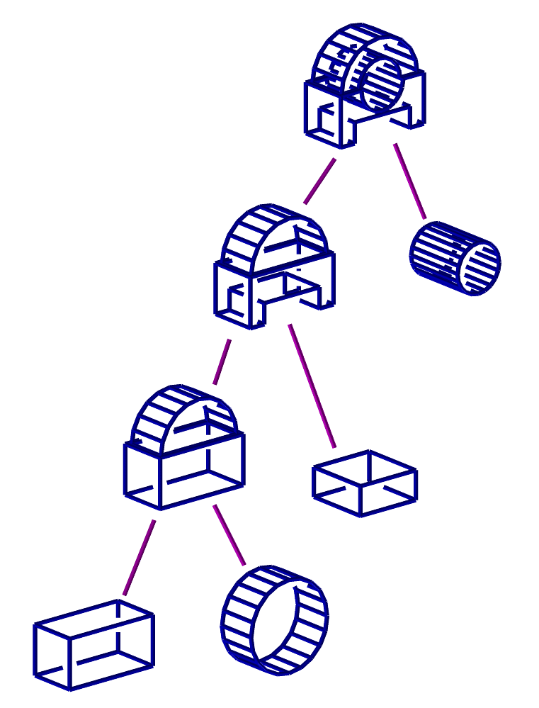
FIGURE: A simple example of a polyhedra model, computed as a sequence of several Boolean operation, presented as a CSG tree.
Example:
    resolution = 20;
    B = box(vector(-1, -1, -0.25), 2, 1.2, 0.5);
    C = con2(vector(0, 0, -1.5), vector(0, 0, 3), 0.7, 0.3);

    D = convex(B - C);
    E = convex(C - B);
    F = convex(B + C);
    G = convex(B * C);

    tr = rotx( -90 ) * roty( 40 ) * rotx( -30 );

    All = list( D * tr * trans( vector(  0.6,  0.5, 0.0 ) ),
                E * tr * trans( vector(  3.0,  0.0, 0.0 ) ),
                F * tr * trans( vector( -2.0,  0.0, 0.0 ) ),
                G * tr * trans( vector(  0.7, -1.0, 0.0 ) ) )
            * scale( vector( 0.25, 0.25, 0.25 ) )
            * trans( vector( -0.1, -0.3, 0.0 ) );
    view_mat = rotx( 0 );
    view( list( view_mat, All ), on );
    save( "booleans", list( view_mat, All ) );
This is a complete example of how to compute the union, intersection and both differences of a box and a truncated cone.
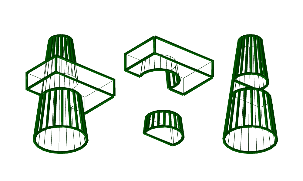
FIGURE: Geometric Boolean operations between a box and a truncated cone. Shown are union (left), intersection (bottom center), box minus the cone (top center), and cone minus the box (right).
Special cases can be very difficult to handle when considering Boolean operations. Consider an axes parallel bounding cube. Consider a second cube rotated alpha degrees from the first cube. At large angles, the Boolean operations are fairly simple to compute. Nevertheless, as alpha approaches zero, the almost coplanar planes of the two intersecting cubes make it very difficult to robustly and consistently compute their intersection.
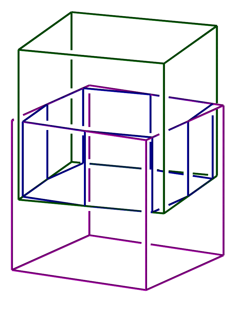
FIGURE: Examples of robustness of Boolean Intersection operation. As the rotation anlge approaches zero, the coplanarity of the intersecting models puts very difficult constraints on the robustness of the result. In this specific example, using IRIT, the operation fails at angles of 10e-6 and below.
There are several flags to control the Boolean operations. See IRITSTATE command for the "InterCrv", "InterUV", "Coplanar", and "PolySort" states.
Priority of operators
The following table lists the priority of the different operators.| Lowest | Operator | Name of operator |
|---|---|---|
| priority | , | comma |
| : | colon | |
| &&, || | logical and, logical or | |
| =,==,!=,<=,>=,<,> | assignment, equal, not equal, less | |
| equal, greater equal, less, greater | ||
| +, - | plus, minus | |
| *, / | multiply, divide | |
| Highest | ^ | power |
| priority | -, ! | unary minus, logical not |
Grammar
The grammar of the IRIT parser follows guidelines similar to those of the C language for simple expressions. However, complex statements differ. See the IF, FOR, FUNCTION, and PROCEDURE below for the usage of these clauses.Function Description
NumericType returning functions
ABS
NumericType ABS( NumericType Operand )
returns the absolute value of the given Operand.
ACOS
NumericType ACOS( NumericType Operand )
returns the arc cosine value (in radians) of the given Operand.
AREA
 NumericType AREA( PolygonType Object )

 or

 NumericType AREA( CurveType Object )
returns the area of the given Object (in object units).
ASIN
NumericType ASIN( NumericType Operand )
returns the arc sine value (in radians) of the given Operand.
ATAN
NumericType ATAN( NumericType Operand )
returns the arc tangent value (in radians) of the given Operand.
ATAN2
NumericType ATAN2( NumericType Operand1, NumericType Operand2 )
returns the arc tangent value (in radians) of the given ratio: Operand1 / Operand2, over the whole circle.
COS
NumericType COS( NumericType Operand )
returns the cosine value of the given Operand (in radians).
CLNTEXEC
NumericType CLNTEXEC( StringType ClientName )
Initiate communication channels to a client named ClientName. ClientName is executed by this function as a sub process. Two communication channels are opened between the IRIT server and the new client, for read and write. See also CLNTCRSR, CLNTREAD, CLNTWRITE, and CLNTCLOSE. If ClientName is an empty string, the user is provided with the new communication port to be used and the server blocks for the user to manually execute the client after setting the proper IRIT_SERVER_HOST/PORT environment variables.
Example:
   h1 = CLNTEXEC( "" );
   h2 = CLNTEXEC( "nuldrvs -s-" );
executes two clients, one named nuldrvs while the other one is prompted for by the user. As a result of the second invokation of CLNTEXEC, the user will be prompted with a message similar to:
    Irit: Startup your program - I am waiting...

    setenv IRIT_SERVER_PORT 2182
and he/she will need to set the proper environment variable and execute their client manually.
CPOLY
NumericType CPOLY( PolygonType Object )
returns the number of polygons in the given polygonal Object.
DSTPTLN
NumericType DSTPTLN( PointType Pt, PointType LineOrig, VectorType LineRay )
returns the distance between a given point Pt and line LineOrig, LineRay. See also PTPTLN.
DSTPTPLN
NumericType DSTPTPLN( PointType Pt, PlaneType Plane )
returns the distance between a given point Pt and plane Plane.
DSTLNLN
 NumericType DSTLNLN( PointType Line1Orig, VectorType Line1Ray,
                      PointType Line2Orig, VectorType Line2Ray )
returns the distance between two lines defined by point LineiOrig and ray LineiRay. See also PTSLNLN.
EXP
NumericType EXP( NumericType Operand )
returns the natural exponential value of the given Operand.
FLOOR
NumericType FLOOR( NumericType Operand )
returns the largest integer not greater than the Operand.
FMOD
NumericType FMOD( NumericType Operand, NumericType Mod )
returns the floating point remainder of the division of the Operand by Mod.
LN
NumericType LN( NumericType Operand )
returns the natural logarithm value of the given Operand.
LOG
NumericType LOG( NumericType Operand )
returns the base 10 logarithm value of the given Operand.
MESHSIZE
NumericType MESHSIZE( FreeformType Freeform, ConstantType Direction )
returns the size of the Freeform's mesh in a Direction, which will be COL, ROW or DEPTH. For the case of a multivariate Freeform, the Direction is an integer value starting from 0. See also FFMSIZE. Examples:
   Len = MESHSIZE( Crv, COL );
   RSize = MESHSIZE( Sphere, ROW );
   CSize = MESHSIZE( Sphere, COL );
   TVSize = MESHSIZE( TV, COL ) * MESHSIZE( TV, ROW ) * MESHSIZE( TV, DEPTH );
   MVSize1 = MESHSIZE( MV, 1 );
POWER
NumericType POWER( NumericType Operand, NumericType Exp )
returns the Operand to the power of Exp.
RANDOM
NumericType RANDOM( NumericType Min, NumericType Max )
returns a randomized value between Min and Max. See also "RandomInit", in the IRITSTATE function.
SIN
NumericType SIN( NumericType Operand )
returns the sine value of the given Operand (in radians).
SIZEOF
 NumericType SIZEOF( PointTypr Pt | VectorType Vec | PlaneType Pln |
                     CtlPtType CtlPt | ListType List | PolygonType Poly |
                     CurveType Crv | StringType Str )
returns the size of a point, vector, plane, or control point (negative size if rational) or the length of a list if List, the number of polygons if Poly, the length of the control polygon if Crv, or the number of characters in string if Str. If, however, only one polygon is in Poly, it returns the number of vertices in that polygon.
Example:
   len = SIZEOF( list( 1, 2, 3 ) );
   numPolys = SIZEOF( axes );
   numCtlpt = SIZEOF( circle( vector( 0, 0, 0 ), 1 ) );
will assign the value of 3 to the variable len, set numPolys to the number of polylines in the axes object, and set numCtlPt to 9, the number of control points in a circle.
SQRT
NumericType SQRT( NumericType Operand )
returns the square root value of the given Operand.
TAN
NumericType TAN( NumericType Operand )
returns the tangent value of the given Operand (in radians).
THISOBJ
NumericType THISOBJ( StringType Object )
returns the object type of the given name of an Object. This can be one of the constants,
| UNDEF_TYPE | PLANE_TYPE | CTLPT_TYPE | MODEL_TYPE |
|---|---|---|---|
| POLY_TYPE | MATRIX_TYPE | LIST_TYPE | VMODEL_TYPE |
| NUMERIC_TYPE | CURVE_TYPE | TRIVAR_TYPE | MULTIVAR_TYPE |
| POINT_TYPE | SURFACE_TYPE | TRISRF_TYPE | |
| VECTOR_TYPE | STRING_TYPE | TRIMSRF_TYPE |
VOLUME
NumericType VOLUME( PolygonType Object )
returns the volume of the given Object (in object units). It returns the volume of the polygonal object, not the volume of the object it might approximate.
This routine decomposes all non-convex polygons to convex ones, as a side effect (see CONVEX).
GeometricType returning functions
ACCESSANLZ
AnyType ACCESSANLZ( NumericType Operation, ListType Params )
This function performs patch (sub-surface) ray accessilibty operations based on the first Operation parameter and the given direction and surface(s), etc. parameters in Params.
If Operation is 1, the analysis is initialized. The Params in this case are a list, containing a list of surfaces followed by the requested size for the patch subdivision, the minimum size for the patch subdivision, the requested normal cone span of the patch, and the cropping applied to the surfaces (in paramteric domain values).
Size refers to the longest dimension of the sub-surface bounding box. The result is that the supplied surfaces will be subdivided into patches with a size that is between the maximum and minimum sizes, and unless the minimum size is reach will have a normal cone span that is less than the requested value. The returned value is the number of patches created.
If Operation is 2, all the create patches (subsurfaces) are retrieved. The returned value are the patches. Params is nil here.
For Operation equal 3, all accessible patches from a given direction (and paramters) are retrieved. In this operation, Params are first the direction, which is the 'up' axis from which accessiblity is determined, folowed by an angular span, and position span. The angular span means all rays in a cone (with the given angle) are checked, the position span adds all rays emenating from a circle with the given radius (aligned to the direction) are also tested. The returned value are the accessible patches.
Finally, if Operation is 9, all auxiliary data is freed. Params is nil and Zero is returned.
Example:
  # Operation = 1: Initializes accessibility - subdivide the input surfaces.
  # Parameter list( Srfs, RequestSize, MinimalSize, NormalAngluarSpan,
  #                 CropSrfBndryEps )
  A = AccessAnlz( 1, list( AlphaSrf, 0.05, 5.0, 0.01, 0.0 ) );

  # Operation = 2: Inspect all subdivided patches.
  # Parameter list()   (empty list)
  AllPatches = AccessAnlz( 2, nil() );

  # Operation = 3: Query the qaccessible patches from the prescribed direction.
  # Parameter list( AccessDir, RotationDeviation, TranslationDeviation )
  # Also moves the accessible patches a tad in v to avoid Z fighting:
  v = vector( 0, 0, 1 );
  AllAccessiblePatches1 = AccessAnlz( 3, list( v, 0.1, 0.01 ) ) *
                                                     trans( v * sc( 0.002 ) );

  # Operation = 9: Free all allocations and data structure.
  # Parameter list()   (empty list)
  A = AccessAnlz( 9, nil() );
ALGPROD
 SurfaceType ALGPROD( CurveType Crv1, CurveType Crv2 )

 or

 TrivarType ALGPROD( CurveType Crv1, SurfaceType Srf2 )
Given two curves (or a curve and a surface), computes a surface (trivariate) that is their algebraic product:
S(u, v) = C1(u) * C2(v)or
T(u, v, w) = C1(u) * S2(v, w)
Example:
 c1 = circle( vector( 0.0, 0.0, 0.2 ), 0.7 );
 c2 = ctlpt( E3, -0.2, -0.5, -1.5 ) + ctlpt( E3, 0.2, 0.5, 1.5 );

 s = algprod( c1, c2 );
ALGSUM
 SurfaceType ALGSUM( CurveType Crv1, CurveType Crv2 )

 or

 TrivarType ALGSUM( CurveType Crv1, SurfaceType Srf2 )
Given two curves (or a curve and a surface), computes a surface (trivariate) that is their algebraic sum:
S(u, v) = C1(u) + C2(v)or
T(u, v, w) = C1(u) + S2(v, w)
Example:
 c1 = circle( vector( 0.0, 0.0, 0.0 ), 0.7 );
 c2 = ctlpt( E3, -0.2, -0.5, -1.5 ) + ctlpt( E3, 0.2, 0.5, 1.5 );

 s1 = algsum( c1, c2 );

 c2 = cbspline( 3,
                list( ctlpt( E3, 0.0, 0.0, 0.0 ),
                      ctlpt( E3, 0.0, 0.0, 0.7 ),
                      ctlpt( E3, 0.0, 1.5, 1.0 ),
                      ctlpt( E3, 0.0, 0.0, 1.3 ),
                      ctlpt( E3, 0.0, 0.0, 2.0 ) ),
                list( KV_OPEN ) );

 s2 = algsum( c1, c2 );
creates two algebraic sum surfaces, one in the shape of a cylinder as a sum of a line and a circle, and one circular sweep like. See figure for an example.

FIGURE: An algebraic sum of a circle and a line creating a cylinder (left) and a general sweep like surface (right), both using ALGSUM.
AMFIBER3AXIS
 ListType AMFIBER3AXIS( CurveType FiberCrv | ListType FiberCrvs,
                        CurveType AmbientCrv | ListType AmbientCrvs,
                        NumericType MinDist, NumericType Accuracy,
                        NumericType PrintRadius, NumericType ExtXYRadius,
                        NumericType ExtAngle, NumericType ZOffset,
                        NumericType Invert )
computes proper ordering of 3D printing of ambient print path curves along with (strengthening) fibers. FiberCrv(s) holds the input fiber print paths, where as AmbientCrv(s) holds the ambient print path curves. MinDist sets the minimal distance to allow between fiber and ambient curves when we subtract the fiber volume from the ambient curves. Accuracy controls the accuracy of the space subdivision process. PrintRadius defines the radius of the extruded materials while ExtXYRadius defines the bottom width of the extruder bounding frustum (for accessibility considerations). ExtAngle sets the extruders' bounding frustum angle. ZOffset sets the Z vertical offset of the extruder above the deposited material. Finally, Invert TRUE will return only the regions of the ambient curves that were subtracted from the fiber curves, for mostly debugging purposes.
Example:
 TPath = AMFiber3Axis( FiberCrvs, AmbientCrvs, SubWidth, Accuracy,
                       PrintRadius, XYRadius, Angle, ZOffs, Invert );
ANALYFIT
 ListType ANALYFIT( ListType UVPts, ListType EucPts,
                    NumericType FirstAtOrigin, NumericType Degree )
computes a surface fit to the given paraametrized points data. The fitted surface will be of bi-degree Degree, fitting points EucPts at parameters UVPts. Needless to say EucPts and UVPts should be lists of points of similar length. If FirstAtOrigin is TRUE, all points are translated so the first point in EucPts is at the origin. Only the first coordinates of UVPts are used.
Example:
    Fitting = nil();
    Eps = 1e-2;

    PtPln = nil():
    for (i = 1, 1, 100,
        snoc( point( random( -1, 1 ), random( -1, 1 ), random( -Eps, Eps ) ),
              PtPln ) );

    BilinCoefs = ANALYFIT( PtPln, PtPln, 0, 1 ) );
fits a bilinear to the given planar data with noise. See also the COERCE function from POWER_TYPE to BEZIER_TYPE, and FITPMODEL.
ANIMEVAL
AnyType ANIMEVAL( NumericType Time, AnyType Object, NumericType EvalMats )
evaluates the animation curves in Object at time Time. The transformations for time Time are saved at the respective sub objects of Object as "animation_mat" matrices, if EvalMats is TRUE. If, however, EvalMats is FALSE, the evaluated/mapped geometry is returned directly.
For example,
    mov_x = cbezier( list( ctlpt( E1, 0.0 ), ctlpt( E1, 1.0 ) ) );
    attrib( axes, "animation", list( mov_x ) );
    axes2 = ANIMEVAL( 0.5, axes, true );
and axes2 will have a matrix in attribute "animation_mat" of translation in x of 1/2.
ANTIPODAL
 ListType ANTIPODAL( CurveType Crv, NumericType SubdivTol,
                                    NumericType NumerTol )

 or

 ListType ANTIPODAL( SurfaceType Srf, NumericType SubdivTol,
                                      NumericType NumerTol )
computes distinct antipodal pairs on curve Crv or on surface Srf. An antipodal pair defines two distinct locations on Crv or on Srf that a line through the two locations is orthogonal to the tangent space of the shape, at thouse locations. In other words, the normals to the freeform shape at those two locations are along the line connecting the locations. SubdivTol and NumerTol control the tolerance of the computation as in MZERO.
Examples:
A = ANTIPODAL( Srf, 1e-3, -1e-12 );
AOFFSET
 CurveType AOFFSET( CurveType Crv, NumericType OffsetDistance,
                    NumericType Epsilon, NumericType TrimLoops,
                    NumericType BezInterp )

 or

 CurveType AOFFSET( CurveType Crv, CurveType OffsetDistance,
                    NumericType Epsilon, NumericType TrimLoops,
                    NumericType BezInterp )
computes an offset of OffsetDistance with a globally bounded error (controlled by Epsilon). The smaller Epsilon is, the better the approximation to the offset. The bounded error is achieved by adaptive refinement of the Crv. If OffsetDistance is a (scalar) curve, the curve's first coordinate is used to prescribe a variable offset amount along the curve. Both Crv and OffsetDistance must share the same parametric domain. If TrimLoops is TRUE or on, the regions of the object that self-intersect as a result of the offset operation are trimmed away. If BezInterp is TRUE, each curve's segment is interpolated instead of approximated.
Example:
    OffCrv1 = AOFFSET( Crv, 0.5, 0.01, FALSE, FALSE );
    OffCrv2 = AOFFSET( Crv, 0.5, 0.01, TRUE, FALSE );
computes an adaptive offset to Crv with OffsetDistance of 0.5 and Epsilon of 0.01 and trims the self intersection loops in the second instance. See also OFFSET, TOFFSET, LOFFSET, and MOFFSET. See figure for an example.
FIGURE: Adaptive offset approximation (thick) of a B-spline curve (thin). On the left, the self intersections in the offset computed in the right are eliminated. Both offsets were computed using AOFFSET.
ARC
CurveType ARC( VectorType StartPos, VectorType Center, VectorType EndPos )
constructs an arc between the two end points StartPos and EndPos, centered at Center. THe arc will always be less than 180 degrees, so the shortest circular path from StartPos to EndPos is selected. The case where StartPos, Center, and EndPos are collinear is illegal, since it attempts to define a 180 degrees arc. The arc is constructed as a single rational quadratic Bezier curve.
Example:
    Arc1 = ARC( vector( 1.0, 0.0, 0.0 ),
                vector( 1.0, 1.0, 0.0 ),
                vector( 0.0, 1.0, 0.0 ) );
constructs a 90 degrees arc, tangent to both the X and Y axes at coordinate 1. See figure for an example.
FIGURE: A 90 degree arc constructed using the ARC constructor (left) and a 280 degrees arc (right) constructed using the ARC360 constructor.
See also ARC360
ARC360
 CurveType ARC360( VectorType Center, NumericType Radius,
                   NumericType StartAngle, NumericType EndAngle )
constructs an arc between the two angles (degrees) StartAngle and EndAngle, centered at Center. The arc will always be less than 360 degrees. The arc is constructed as a rational quadratic B-spline curve.
Example:
Arc2 = ARC360( vector( 0.0, 0.0, 0.0 ), 1.0, 75, 355 );
constructs a 280 degrees arc. See figure for an example. See also ARC.
AREPARAM
AnyType AREPARAM( AnyType Obj, NumericType Min, NumericType Max )
Updates the time domain of the animation embedded in Obj to be from Min to Max. This function has an effect only if Obj has animation(s) set for it. See the Animation section and ATTRIB to set animation attributes on objects.
Example:
ASrf = AREPARAM( Srf, 0, 2 );
Sets the animation time to be from zero to two time units.
BBOX
ListType BBOX( GeometricTreeType Geom )
Given a (tree of) geometry, Geom computes its bounding box and return it as a list of six numbers: XMin/Max, YMin/Max, ZMin/Max, in this order.
Example:
B1 = BBOX( axes );
BELTCURVE
 ListType BELTCURVE( PolyType Pulleys, NumericType Thickness,
                     NumericType BoundingArcs, NumericType ReturnCrvs )
Computes a belt for a given set of Pulleys defined as point list of the form (x, y, r) for each Pulley. Positive r designates a CW pulley whereas a negative r designates a CCW pulley. The thickness of the belt is defined by Thickness. BoundingArcs is usually zero but if not, prescribes two bounding arcs for each linear segment of the belt. ReturnCrvs should be TRUE to simply return the two boundary curves of the belt or FALSE to return a list of arcs/lines of the belt.
Example:
 B1 = BeltCurve( list( vector( 0, 0,   0.6 ),
                       vector( 1, 3,  -0.24 ),
                       vector( 3, 3,  -0.24 ),
                       vector( 3, 1,   0.4 ),
                       vector( 3, -1,  0.3 ),
                       vector( 1, -1,  0.3 ),
                 BeltThickness, CreateBoundingArcs, ReturnCrvs ),
See figure for an example.
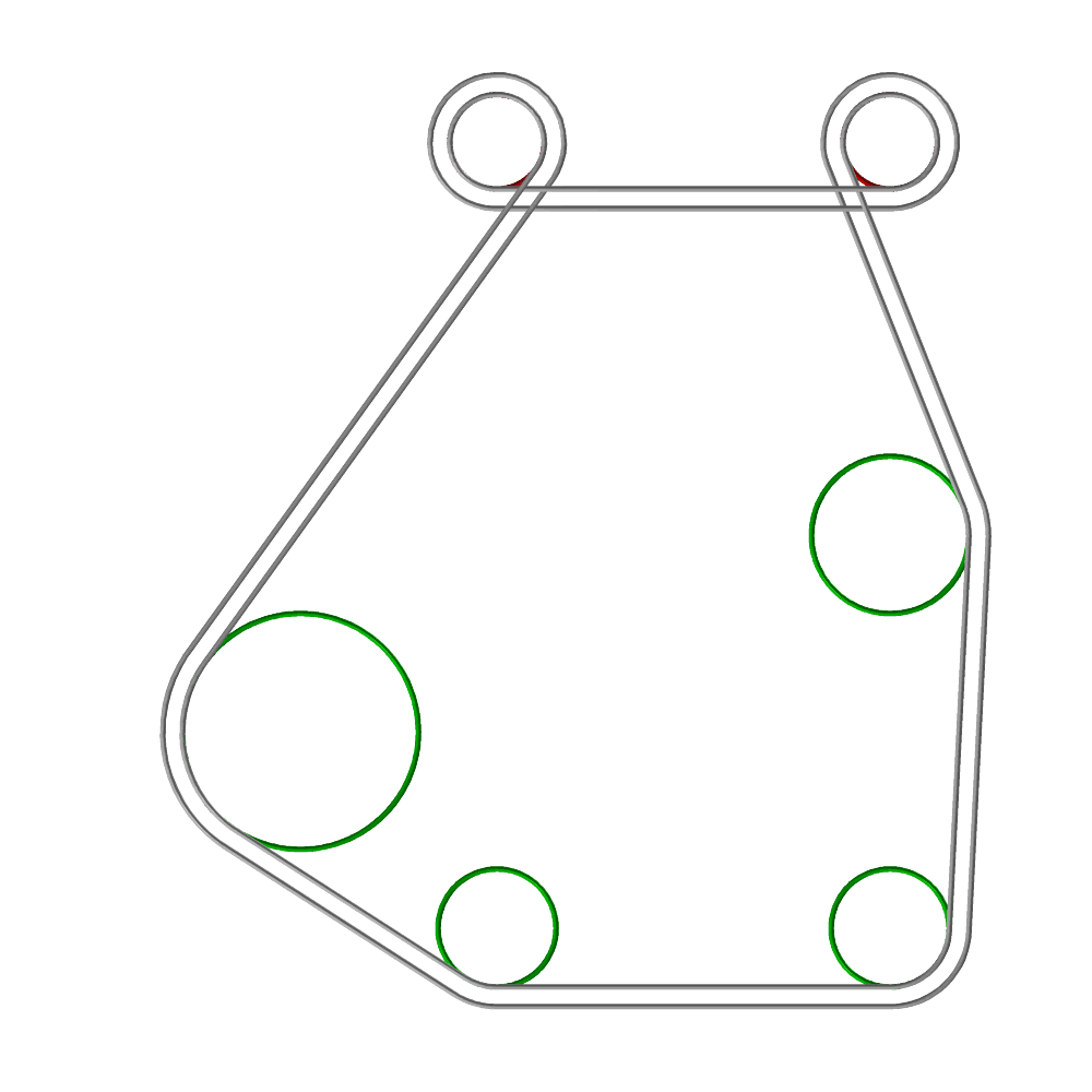
FIGURE: A belt defined using the BELTCURVE function.
BFROM2IMG
 ListType BFROM2IMG( StringType Img1, StringType Img2,
                     NumericType DitherSize, NumericType MatchWidth,
                     NumericType Positive, NumericType AugmentContrast,
                     NumericType SpreadMethod, NumericType SphereRadius )
Constructs a 3D dithering cloud of blobs that looks like Img1 from one view direction and like Img2 from another view direction. DitherSize sets the 3D dithering size - 2, 3, or 4 for 2x2x2, 3x3x3 or 4x4x4. MatchWidth constraints the (bipartitte graph) matching between two rows in the two different images and is measured in pixels. If Positive is true, the images are processed as is. If false, the images are negated first. AugmentContrast allows control over contrast at the cost of more computation, or zero to disable. SpreadMethod is typically true to allow random spreading. SphereRadius sets the radius of the constructed blobs.
See figure for an example.
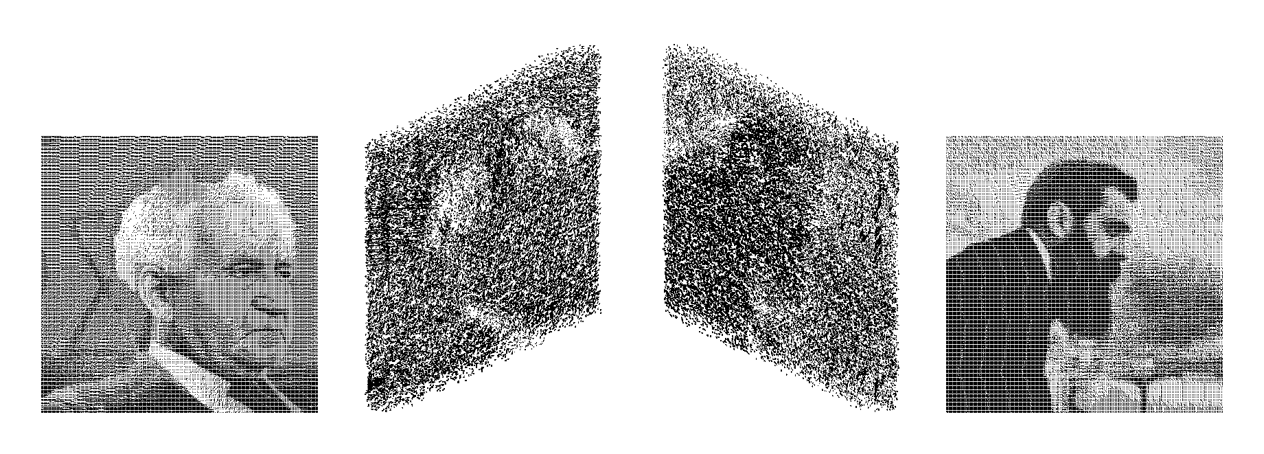
FIGURE: A 3D dithering of two (three) images that creates a cloud of 3D points using the BFROM2IMG (BFROM3IMG) function. Herzl is seen from one view and Ben Gurion from another view.
Example:
    PTS = BFrom2Img( "BenGurion.ppm", "Herzl.ppm",
                     2, 21, true, 0, 2, 0.0 );
constructs a could of points that looks like Herzl from one view and Ben Gurion from another. See also BFROM3IMG, MFROM2IMG, MFROM3IMG, and DTRBYCRVS and DITHER.
BFROM3IMG
 ListType BFROM3IMG( StringType Img1, StringType Img2, StringType Img3,
                     NumericType DitherSize, NumericType MatchWidth,
                     NumericType Positive, NumericType AugmentContrast,
                     NumericType SpreadMethod, NumericType SphereRadius )
Constructs a 3D dithering cloud of blobs that looks like Img1 from one view direction, like Img2 from another view direction, and like Img3 from a third view direction. DitherSize sets the 3D dithering size - 2, 3, or 4 for 2x2x2, 3x3x3 or 4x4x4. MatchWidth constraints the (bipartitte graph) matching between two rows in the two different images and is measured in pixels. If Positive is true, the images are processed as is. If false, the images are negated first. AugmentContrast allows control over contrast at the cost of more computation, or zero to disable. SpreadMethod is typically true to allow random spreading. SphereRadius sets the radius of the constructed blobs.
Example:
    PTS = BFrom2Img( "BenGurion.ppm", "Herzl.ppm", "Rabin.ppm",
                     2, 21, true, 0, 2, 0.0 );
constructs a could of points that looks like Herzl from one view, Ben Gurion from another, and Rabin from a third view. See also BFROM2IMG, MFROM2IMG, and MFROM3IMG.
BFZEROS
 ListType BFZEROS( CurveType Crv, NumericType Axis, NumericType RInit,
                   NumericType NumericTol, NumericType SubdivTol )
computes the zeros of the given univariate Bezier Crv in direction Axis by factoring out t and (1-t) at the found roots. NRInit can be 0 in which case initial roots are set at the middle of the domain, while 1 and 2 starts with initial roots by intersection of the control polygon. With 1 the most middle initial root is used. With 2 the first found initial root is used.
Example:
Zrs = bfzeros( Crv, 1, 0, 1e-10, 1e-4 );
computes the zeros of Crv in the X axis. See also MZERO.
BLND2SRFS
 SurfaceType BLND2SRFS( SurfaceType Srf1, SurfaceType Srf2,
                        NumericType BlendDegree, NumericType TanScale )
constructs a new surface that blends Srf1 at UMin and Srf2 at UMax. BlendDegree can be 2 in which case the blending surface is C^0 continuous (to Srf1 and Srf2) or 4 to achieve C^1 continuity. Finally TanScale controls the strength of the tangential field, if C^1 is sought.
Example:
BSrf = BLND2SRFS( Srf1, Srf2, 4, 1.0 );
See also HERMITE, BLHERMITE and BLSHERMITE
BLHERMITE
 SurfaceType BLHERMITE( CurveType Bndry1, CurveType Bndry2,
                        CurveType Tan1, CurveType Tan2,
                        CurveType Sctn, CurveType Nrml )
computes a Hermite blend surface that supports an arbitrary cross section. This constructs a surface between Bndry1 and Bndry2 so that the first derivative continuity constraints, as prescribed by Tan1 at Bndry1 and Tan2 at Bndry2, are preserved. In addition, the interior between Bndry1 and Bndry2 will follow the shape of planar cross section curve Sctn and will be oriented along the vector field prescribed by Nrml. Cross section Sctn is a planar curve that must start at (-1, 0) and end at (1, 0), and have zero speed at the ends (first control point equals the second and is the same at the end).
Example:
 c1 = ctlpt( e3, 0, 0, 0 ) + ctlpt( e3, 0, 1, 0 );
 c2 = ctlpt( e3, 1, 0, 0 ) + ctlpt( e3, 1, 1, 0 );
 d1 = ctlpt( e3,  1, 0,  1 ) + ctlpt( e3,  1, 0,  0.1 );
 d2 = ctlpt( e3,  1, 0, -0.1 ) + ctlpt( e3,  1, 0, -1 );

 s1 = hermite( c1, c2, d1, d2 );
 color( s1, red );

 cSec = cbspline( 3,
                  list( ctlpt( e2, -1,    0 ),
                        ctlpt( e2, -1,    0 ),
                        ctlpt( e2, -0.14, 0.26 ),
                        ctlpt( e2, -0.65, 0.51 ),
                        ctlpt( e2,  0,    0.76 ),
                        ctlpt( e2,  0.65, 0.51 ),
                        ctlpt( e2,  0.14, 0.26 ),
                        ctlpt( e2,  1,    0 ),
                        ctlpt( e2,  1,    0 ) ),
                  list( kv_open ) );
 n = ctlpt( e3, 0, 0, 1 ) + ctlpt( e3, 0, 0, 1 );

 s2 = BLHERMITE( c1, c2, d1, d2, cSec2, n );
 color( s2, yellow );
constructs a regular Hermite surfaces s1 and a blending Hermite that follows the cross section cSec. See also HERMITE and BLSHERMITE. See figure for an example.
BLSHERMITE
 SurfaceType BLSHERMITE( SurfaceType Srf, CurveType PCrv,
                         CurveType Sctn, NumericType TanScale,
                         AnyType Width, AnyType Height )
computes a Hermite blend surface on Srf along parametric curve of Srf, PCrv, the cross section Sctn, a tangent field scale control TanScale, and the width and height control of Width and Height. Width and Height can be either a numeric value of expected width and height or a scalar field curve prescribing the expected width and height along the constructed blend.
The constructed surface, which is C1 continuous to Srf, is positioned along PCrv, a curve in the parametric domain of Srf. The cross section Sctn is a planar curve that must start at (-1, 0) and end at (1, 0), and have zero speed at the ends (first control point equals the second and is the same at the end). TanScale controls how rapid the change in the tangent is, as we move away from the surface.
Example:
 cSec = cbspline( 3,
                  list( ctlpt( e2, -1,    0 ),
                        ctlpt( e2, -1,    0 ),
                        ctlpt( e2, -0.5,  0.2 ),
                        ctlpt( e2, -0.7,  0.3 ),
                        ctlpt( e2,  0,    0.5 ),
                        ctlpt( e2,  0.7,  0.3 ),
                        ctlpt( e2,  0.5,  0.2 ),
                        ctlpt( e2,  1,    0 ),
                        ctlpt( e2,  1,    0 ) ),
                  list( kv_open ) );

 s = -surfPRev( cregion( pcircle( vector( 0, 0, 0 ), 1 ),
                         0, 2 ) * rx( 90 ) );

 s1 = BLSHERMITE( s, ctlpt( E2, 0, 1 ) + ctlpt( E2, 4, 1 ),
                  cSec, 1, 0.2, 0.5 );
 s2 = BLSHERMITE( s, ctlpt( E2, 0, 1.5 ) + ctlpt( E2, 4, 1.5 ),
                  cSec, 0.1, 0.2, 0.5 );
 s3 = BLSHERMITE( s, ctlpt( E2, 0, 0.3 ) + ctlpt( E2, 4, 0.3 ),
                  cSec, 1.5, 0.2, 0.5 );
places three Hermite blend surfaces s1, s2, s3 using the cross section cSec on a unit sphere s. See also HERMITE and BLHERMITE. See figure for an example.
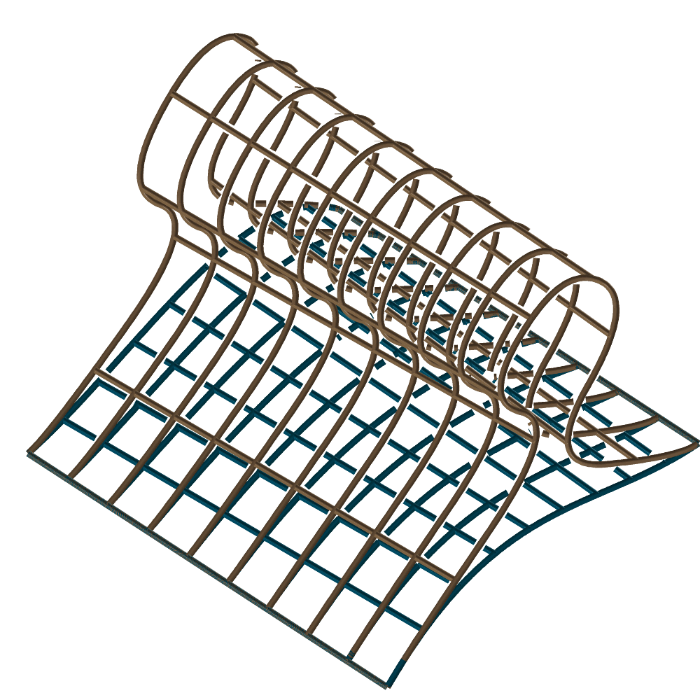
FIGURE: Blending Hermite with a prescribed cross section (left) using BLHERMITE and blending Hermite with a prescribed cross section on a surface (right) using BLSHERMITE.
BLOSSOM
 CtlPtType BLOSSOM( CurveType Crv, ListType BlossomVals )

 or

 CtlPtType BLOSSOM( SurfaceType Srf, ListType BlossomVals )
computes the blossom of the given Crv or Srf and the given blossom values BlossomVals. For a Crv, BlossomVals is expected to hold a linear list of blossom values. For a Srf, BlossomVals is expected to hold two linear lists (for u and v) of blossom values.
Example:
 c1 = cbezier( list( ctlpt( E2, 1.7, 0.0 ),
                     ctlpt( E2, 0.7, 0.7 ),
                     ctlpt( E2, 1.7, 0.3 ),
                     ctlpt( E2, 1.5, 0.8 ),
                     ctlpt( E2, 1.6, 1.0 ) ) );

 BLOSSOM( c1, list( 0, 0, 0, 0 ) ) == coord( c1, 0 ) &&
 BLOSSOM( c1, list( 0, 0, 0, 1 ) ) == coord( c1, 1 ) &&
 BLOSSOM( c1, list( 0, 0, 1, 1 ) ) == coord( c1, 2 ) &&
 BLOSSOM( c1, list( 0, 1, 1, 1 ) ) == coord( c1, 3 ) &&
 BLOSSOM( c1, list( 1, 1, 1, 1 ) ) == coord( c1, 4 );
extracts the control points of an quadric Bezier curve via blossoming and compares this to the results obtained via a traditional extraction approach (via the COORD function).
BOOLONE
SurfaceType BOOLONE( CurveType Crv )
Given a closed curve, the curve is subdivided into four segments equally spaced in the parametric space that are fed into BOOLSUM. This is useful if a surface should "fill" the area enclosed by a closed curve.
Example:
Srf = BOOLONE( circle( vector( 0.0, 0.0, 0.0 ), 1.0 ) );
creates a disk surface containing the area enclosed by the unit circle. See figure for an example.
FIGURE: A Boolean sum of a circle creates a disk (left) using BOOLONE and a general Boolean sum of four curves (right) using BOOLSUM.
See also BOOLSUM and TBOOLONE
BOOLSUM
 SurfaceType BOOLSUM( Mode,
                      CurveType Crv1, CurveType Crv2,
                      CurveType Crv3, CurveType Crv4 )
The Mode parameter indicates which variant of this operator to use. For regular ruling operator, it should be 0. The regular operator constructs a surface using the provided two or four curves as its two/four boundary curves. Curves do not have to have the same order or type, and will be promoted to their least common denominator. In the case of two curves, Crv1 and Crv2 should share an end point and in this case, Crv3 and Crv4 should be a non-curve objects. In the case of four curves, the four curves should form a topological square and match end points and, in principle, be oriented as Left, Right, Top and Bottom boundaries in order. Practically, the curve ordering is not relevant - Crv1 will be picked as Left and the rest three curves will be matched accordingly. Matching of end points is required.
For Kernel-based Boolean sum operator, which is used to construct valid planar Boolean sum surface (aiming to ensure positive Jacobian throughout the domain, the Mode parameter should be a list of five numeric values: ( Op, DistRatio, Limit, SubEps, IsSingular), where
Op is either 0 or 1 for adding DOFs using degree raising or knot insertion, respectively.
DistRatio is a number in [0, 1] to set how far to move internal control points toward the kernel. If 1 the points are moved to the kernel point.
Place a Limit on the number of knots to add or the maximal degree in degree raising.
SubEps is the Subdivision epsilon. 0.01 is a reasonable start for a unit size geometry.
IsSingular can be: TRUE to allow singularity at the kernel point. FALSE all the surface is regular.
Example:
    Cbzr1 = cbezier( list( ctlpt( E3, 0.1, 0.1, 0.1 ),
                           ctlpt( E3, 0.0, 0.5, 1.0 ),
                           ctlpt( E3, 0.4, 1.0, 0.4 ) ) );
    Cbzr2 = cbezier( list( ctlpt( E3, 1.0, 0.2, 0.2 ),
                           ctlpt( E3, 1.0, 0.5, -1.0 ),
                           ctlpt( E3, 1.0, 1.0, 0.3 ) ) );
    Cbsp3 = cbspline( 4,
                      list( ctlpt( E3, 0.1,  0.1, 0.1 ),
                            ctlpt( E3, 0.25, 0.0, -1.0 ),
                            ctlpt( E3, 0.5,  0.0, 2.0 ),
                            ctlpt( E3, 0.75, 0.0, -1.0 ),
                            ctlpt( E3, 1.0,  0.2, 0.2 ) ),
                      list( KV_OPEN ) );
    Cbsp4 = cbspline( 4,
                      list( ctlpt( E3, 0.4,  1.0, 0.4 ),
                            ctlpt( E3, 0.25, 1.0, 1.0 ),
                            ctlpt( E3, 0.5,  1.0, -2.0 ),
                            ctlpt( E3, 0.75, 1.0, 1.0 ),
                            ctlpt( E3, 1.0,  1.0, 0.3 ) ),
                      list( KV_OPEN ) );
    Srf1 = BOOLSUM( 0, Cbzr1, Cbzr2, Cbsp3, Cbsp4 );
    Srf2 = BOOLSUM( 0, Cbzr1, Cbsp3, 0, 0 );
See also BOOLONE and TBOOLSUM
    Left = cbezier(
               ist( ctlpt( E2, -1., -1. ),
                    ctlpt( E2, -1.165, -0.689 ),
                    ctlpt( E2, -1.979, 0.5 ),
                    ctlpt( E2, -1.797, 0.821 ),
                    ctlpt( E2, -1., 1. ) ) );
    Right = cbezier(
               list( ctlpt( E2, 1., -1. ),
                     ctlpt( E2, 1.403, -0.346 ),
                     ctlpt( E2, 0.205, 0.366 ),
                     ctlpt( E2, 0.96, -0.277 ),
                     ctlpt( E2, 1., 1. ) ) );
    Top = cbezier(
             list( ctlpt( E2, -1., -1. ),
                   ctlpt( E2, -0.982, -0.007 ),
                   ctlpt( E2, -0.139, -0.778 ),
                   ctlpt( E2, 0.202, -1.867 ),
                   ctlpt( E2, 1., -1. ) ) );
    Bottom = cbezier(
                list( ctlpt( E2, -1., 1. ),
                      ctlpt( E2, -0.986, 0.909 ),
                      ctlpt( E2, -0.819, 1.822 ),
                      ctlpt( E2, -0.105, 1.939 ),
                      ctlpt( E2, 1., 1. ) ) );
    Srf1 = BOOLSUM( 0, Left, right, top, bottom );
    Srf2 = BOOLSUM( list( 0, 1.0, 8, 0.01, FALSE ),
                    Left, right, top, bottom ) * tx( -3 );
constructs a planar Boolean sum surface upon the four quatric Bezier input curves, Left, Right, Top and Bottom. The naive construction causes self intersection. By using the kernel-based Boolean sum operator, the self intersection can be resolved. After adding degree of freedoms to the input curves using either degree raising operator or refinement. In the given example the operator successed after 8 iteration of degree raising.
BOUNDARY
AnyType BOUNDARY( AnyType Obj )
Given a geometric object Obj, let it be a surface, a trimed surface, or a polygonal model, returns the boundary of the shape.
Example:
CBndry = BOUNDARY( Srf );
returns CBndry.
BOX
 PolygonType BOX( VectorType Point,
                  NumericType Dx, NumericType Dy, NumericType Dz )
creates a BOX polygonal object, whose boundary is coplanar with the XY, XZ, and YZ planes. The BOX is defined by Point as base position, and Dx, Dy, Dz as BOX dimensions. Negative dimensions are allowed.
Example:
B = BOX( vector( 0, 0, 0 ), 1, 1, 1);
creates a unit cube from 0 to 1 in all axes.
BSCTCONCN2
 SurfaceType BSCTCONCN2( PointType ConeApx1, VectorType ConeDir1,
                         NumericType ConeAngle1,
                         PointType ConeApx2, VectorType ConeDir2,
                         NumericType ConeAngle2 )
computes the bisector surface of two cones in general position. The cones' apexes can be found in ConeApx1 and ConeApx2 with axes directions ConeDir1 and ConeDir2 and spanning angles of ConeAngle1 and ConeAngle2.
Example:
BisectSrf = BSCTCONCN2( Apx1, Dir1, Ang1, Apx2, Dir2, Ang2 );
See also BSCPCONCON, BSCTCONCYL, BSCTCYLCYL, BSCTCONLN, BSCTCONPL, BSCTCONPT, BSCTCONSPR, BSCTCYLPL, BSCTCYLPT, BSCTCYLSPR, BSCTPLNLN, BSCTPLNPT, BSCTSPRLN, BSCTSPRPL, BSCTSPRPT, BSCTSPRSPR, BSCTTRSPT, BSCTTRSSPR, CALPHASECTOR, CBISECTOR2D, CBISECTOR3D, SBISECTOR,
BSCTCONCON
 SurfaceType | ListType BSCTCONCON( VectorType ConeDir1, NumericType ConeAngle1,
                                    VectorType ConeDir2, NumericType ConeAngle2,
                                    NumericType Size )
computes the bisector surface of two cones that share the same apex. The cones' directions are ConeDir1 and ConeDir2 and the spanning angles of ConeAngle1 and ConeAngle2. ConeDir1 and ConeDir2 must be in the northern hemisphere; i.e. their Z coefficient must be positive. Size controls the portion of the (infinite) bisector actually represented.
Example:
 BisectSrf = BSCTCONCON( vector( 0, 0, 1 ), 50,
                         vector( 0, 0, 1 ), 20, 1.0 );
computes the bisector of two concentric cones, which is also a cone. See also BSCTCONLN, BSCTCONPL, BSCTCONPT, BSCTCONSPR, BSCTCYLPL, BSCPCONCON, BSCTCONCN2, BSCTCONCYL, BSCTCYLPT, BSCTCYLSPR, BSCTPLNLN, BSCTPLNPT, BSCTSPRLN, BSCTSPRPL, BSCTSPRPT, BSCTSPRSPR, BSCTTRSPT, BSCTTRSSPR, CALPHASECTOR, CBISECTOR2D, CBISECTOR3D, SBISECTOR
BSCTCONCYL
 SurfaceType BSCTCONCYL( PointType ConeApx1, VectorType ConeDir1,
                         NumericType ConeAngle1,
                         PointType CylPt2, VectorType CylDir2,
                         NumericType CylRad2 )
computes the bisector surface of a cone and a cylinder in general position. The cones apex is in ConeApx1 with axes direction of ConeDir1 and spanning angles of ConeAngle1. The second cylinder starts at CylPt2, in direction CylDir2 and radius CylRad2.
Example:
BisectSrf = BSCTCONCYL( Apx1, Dir1, Ang1, Pt2, Dir2, Rad2 );
See also BSCPCONCON, BSCTCONCN2, BSCTCYLCYL, BSCTCONLN, BSCTCONPL, BSCTCONPT, BSCTCONSPR, BSCTCYLPL, BSCTCYLPT, BSCTCYLSPR, BSCTPLNLN, BSCTPLNPT, BSCTSPRLN, BSCTSPRPL, BSCTSPRPT, BSCTSPRSPR, BSCTTRSPT, BSCTTRSSPR, CALPHASECTOR, CBISECTOR2D, CBISECTOR3D, SBISECTOR
BSCTCONLN
 SurfaceType | ListType BSCTCONLN( VectorType ConeDir, NumericType ConeAngle,
                                   VectorType LineDir, NumericType Size )
computes the bisector surface of a cone and a line through its apex. The cone's direction is ConeDir and its spanning angle is ConeAngle. ConeDir and LineDir must be in the northern hemisphere; i.e. their Z coefficient must be positive. Size controls the portion of the (infinite) bisector actually represented.
Example:
BisectSrf = ( vector( 0, 0, 1 ), 45, vector( 0, 0.1, 1 ), 1 );
computes the bisector surface of a cone along the Z axis with spanning angle of 45 degrees, and a line through its apex in direction ( 0, 0.1, 1 ).
See also BSCPCONCON, BSCTCONCN2, BSCTCONCYL, BSCTCONCON, BSCTCONPL, BSCTCONPT, BSCTCONSPR, BSCTCYLPL, BSCTCYLPT, BSCTCYLSPR, BSCTPLNLN, BSCTPLNPT, BSCTSPRLN, BSCTSPRPL, BSCTSPRPT, BSCTSPRSPR, BSCTTRSPT, BSCTTRSSPR, CALPHASECTOR, CBISECTOR2D, CBISECTOR3D, SBISECTOR,
BSCTCONPL
 SurfaceType | ListType BSCTCONPL( PointType ConeApex, VectorType ConeDir,
                                   NumericType ConeAngle, NumericType Size )
computes the bisector surface of a general cone and the XY plane (Z = 0 plane). The cone's apex is at ConeApex, the cone's direction is ConeDir and its spanning angle is ConeAngle. Dir must be in the northern hemisphere; i.e. their Z coefficient must be positive. Size controls the portion of the (infinite) bisector actually represented.
Example:
BisectSrf = BSCTCONPL( point( 0, 0, -0.3 ), vector( 1, 1, 1 ), 20, 1 );
computes the bisector surface of a cone with its apex at (0, 0, -0.3) along the axis (1, 1, 1) with spanning angle of 20 degrees, and the plane Z = 0.
See also BSCPCONCON, BSCTCONCN2, BSCTCONCYL, BSCTCONCON, BSCTCONLN, BSCTCONPT, BSCTCONSPR, BSCTCYLPL, BSCTCYLPT, BSCTCYLSPR, BSCTPLNLN, BSCTPLNPT, BSCTSPRLN, BSCTSPRPL, BSCTSPRPT, BSCTSPRSPR, BSCTTRSPT, BSCTTRSSPR, CALPHASECTOR, CBISECTOR2D, CBISECTOR3D, SBISECTOR.
BSCTCONPT
 SurfaceType | ListType BSCTCONPT( PointType ConeApex, VectorType ConeDir,
                                   NumericType ConeAngle, PointType Pt,
                                   NumericType Size )
computes the bisector surface of a cone in a general position and a point, Pt. The cone's apex is at ConeApex, the cone's direction is ConeDir and its spanning angle is ConeAngle. Size controls the portion of the (infinite) bisector actually represented.
Example:
   Bisect = BSCTCONPT( point( 0, 0, 0 ), vector( 0, 0, 1 ), 22,
                       point( 0, 0.2, 0.7 ), 1 );
See also BSCPCONCON, BSCTCONCN2, BSCTCONCYL, BSCTCONCON, BSCTCONLN, BSCTCONPL, BSCTCONSPR, BSCTCYLPL, BSCTCYLPT, BSCTCYLSPR, BSCTPLNLN, BSCTPLNPT, BSCTSPRLN, BSCTSPRPL, BSCTSPRPT, BSCTSPRSPR, BSCTTRSPT, BSCTTRSSPR, CALPHASECTOR, CBISECTOR2D, CBISECTOR3D, SBISECTOR.
BSCTCONSPR
 SurfaceType | ListType BSCTCONSPR( PointType ConeApex, VectorType ConeDir,
                                    NumericType ConeAngle, PointType SptCntr,
                                    NumericType SprRadius, NumericType Size )
computes the bisector surface of a cone and a sphere. The cone's apex is at ConeApex, the cone's direction is ConeDir and its spanning angle is ConeAngle. The sphere is centered at SptCntr and has a radius of SprRadius. Size controls the portion of the (infinite) bisector actually represented.
Example:
    BisectSrf = BSCTCONSPR( point( 0, 0, 0 ), vector( 0, 0, 1 ),
                            45, point( 0, 0, 1 ), 0.5, 2.0 );
computes the bisector between a cone along the Z axis with a 45 degree spanning angle and a sphere at (0, 0, 1) of radius 0.5.
See also BSCPCONCON, BSCTCONCN2, BSCTCONCYL, BSCTCONCON, BSCTCONLN, BSCTCONPL, BSCTCONPT, BSCTCYLPL, BSCTCYLPT, BSCTCYLSPR, BSCTPLNLN, BSCTPLNPT, BSCTSPRLN, BSCTSPRPL, BSCTSPRPT, BSCTSPRSPR, BSCTTRSPT, BSCTTRSSPR, CALPHASECTOR, CBISECTOR2D, CBISECTOR3D, SBISECTOR.
BSCTCYLCYL
 SurfaceType BSCTCYLCYL( PointType CylPt1, VectorType CylDir1,
                         NumericType CylRad1,
                         PointType CylPt2, VectorType CylDir2,
                         NumericType CylRad2 )
computes the bisector surface of two cylinders in a general position. The cylinders start at CylPt1 and CylPt2 and follow the directions CylDir1 and CylDir2. They have radii of CylRad1 and CylRad2.
Example:
BisectSrf = BSCTCYLCYL( Pt1, Dir1, Rad1, Pt2, Dir2, Rad2 );
See also BSCPCONCON, BSCTCONCN2, BSCTCONCYL, BSCTCONLN, BSCTCONPL, BSCTCONPT, BSCTCONSPR, BSCTCYLPL, BSCTCYLPT, BSCTCYLSPR, BSCTPLNLN, BSCTPLNPT, BSCTSPRLN, BSCTSPRPL, BSCTSPRPT, BSCTSPRSPR, BSCTTRSPT, BSCTTRSSPR, CALPHASECTOR, CBISECTOR2D, CBISECTOR3D, SBISECTOR.
BSCTCYLPL
 SurfaceType | ListType BSCTCYLPL( PointType CylPos, VectorType CylDir,
                                   NumericType CylRadius, Size )
computes the bisector surface of a a cylinder and the XY plane (plane Z = 0). The cylinder is located at CylPos, in the direction of CylDir which also sets the length of the cylinder. The radius of the cylinder is CylRadius. Size controls the portion of the (infinite) bisector actually represented.
Example:
    Pt = point( 0.1, 0, 0.2 );
    BisectSrf = BSCTCYLPL( point( 0, 0, 0.5 ), vector( 0, 0, 1 ), 0.2, 1 );
computed the bisector surface between a cylinder of radius 0.2 along the Z axis and the XY plane.
See also BSCPCONCON, BSCTCONCN2, BSCTCONCYL, BSCTCONCON, BSCTCONLN, BSCTCONPL, BSCTCONPT, BSCTCONSPR, BSCTCYLPT, BSCTCYLSPR, BSCTPLNLN, BSCTPLNPT, BSCTSPRLN, BSCTSPRPL, BSCTSPRPT, BSCTSPRSPR, BSCTTRSPT, BSCTTRSSPR, CALPHASECTOR, CBISECTOR2D, CBISECTOR3D, SBISECTOR.
BSCTCYLPT
 SurfaceType | ListType BSCTCYLPT( PointType CylPos, VectorType CylDir,
                                   NumericType CylRadius, PointType Pt,
                                   NumericType Size )
computes the bisector surface of a a cylinder and a point, Pt. The cylinder is located at CylPos, in the direction of CylDir which also sets the length of the cylinder. The radius of the cylinder is CylRadius. Size controls the portion of the (infinite) bisector actually represented.
Example:
    Pt = point( 0.1, 0, 0.2 );
    BisectSrf = BSCTCYLPT( point( 0, 0, 0.5 ), vector( 0, 0, 1 ), 0.2, Pt, 1 );
computes the bisector surface between a cylinder of radius 0.2 along the Z axis and a point at (0.1, 0, 0.2).
See also BSCPCONCON, BSCTCONCN2, BSCTCONCYL, BSCTCONCON, BSCTCONLN, BSCTCONPL, BSCTCONPT, BSCTCONSPR, BSCTCYLPL, BSCTCYLSPR, BSCTPLNLN, BSCTPLNPT, BSCTSPRLN, BSCTSPRPL, BSCTSPRPT, BSCTSPRSPR, BSCTTRSPT, BSCTTRSSPR, CALPHASECTOR, CBISECTOR2D, CBISECTOR3D, SBISECTOR
BSCTCYLSPR
 SurfaceType | ListType BSCTCYLSPR( PointType CylPos, VectorType CylDir,
                                    NumericType CylRadius, PointType SprCntr,
                                    NumericType SprRadius, NumericType Size )
computes the bisector surface of a cylinder and a sphere. The cylinder is located at CylPos, in the direction of CylDir which also sets the length of the cylinder. The radius of the cylinder is CylRadius. The sphere is centered at SptCntr and has a radius of SprRadius. Size controls the portion of the (infinite) bisector actually represented.
Example:
    BisectSrf = BSCTCYLSPR( point( 0, 0, 1.5 ), vector( 0, 0, 3 ), 0.2,
                            point( 0, 0, 0 ), 0.7, 3 );
computed the bisector surface between a cylinder of radius 0.2 along the Z axis and a sphere at the origin with radius 0.7.
See also BSCPCONCON, BSCTCONCN2, BSCTCONCYL, BSCTCONCON, BSCTCONLN, BSCTCONPL, BSCTCONPT, BSCTCONSPR, BSCTCYLPL, BSCTCYLPT, BSCTPLNLN, BSCTPLNPT, BSCTSPRLN, BSCTSPRPL, BSCTSPRPT, BSCTSPRSPR, BSCTTRSPT, BSCTTRSSPR, CALPHASECTOR, CBISECTOR2D, CBISECTOR3D, SBISECTOR.
BSCTPLNLN
SurfaceType | ListType BSCTPLNLN( VectorType LineDir, NumericType Size )
computes the bisector surface of the XY plane (plane Z = 0) and a line in direction LineDir. The plane and the line are assumed to intersect at the origin. Size controls the portion of the (infinite) bisector actually represented.
Example:
BisectSrf = BSCTPLNLN( vector( 0, 0, 1 ), 1 );
computes the bisector of the XY plane and the Z axis (a cone).
See also BSCPCONCON, BSCTCONCN2, BSCTCONCYL, BSCTCONCON, BSCTCONLN, BSCTCONPL, BSCTCONPT, BSCTCONSPR, BSCTCYLPL, BSCTCYLPT, BSCTCYLSPR, BSCTPLNPT, BSCTSPRLN, BSCTSPRPL, BSCTSPRPT, BSCTSPRSPR, BSCTTRSPT, BSCTTRSSPR, CALPHASECTOR, CBISECTOR2D, CBISECTOR3D, SBISECTOR.
BSCTPLNPT
SurfaceType | ListType BSCTPLNPT( PointType Pt, NumericType Size )
computes the bisector surface of the XY plane (plane Z = 0) and a point Pt. This surface is a paraboloid of revolution. Size controls the portion of the (infinite) bisector actually represented.
Example:
BisectSrf = BSCTPLNPT( point( 0, 0, 1 ), 1 );
computes the bisector surface of the XY plane and the point (0, 0, 1).
See also BSCPCONCON, BSCTCONCN2, BSCTCONCYL, BSCTCONCON, BSCTCONLN, BSCTCONPL, BSCTCONPT, BSCTCONSPR, BSCTCYLPL, BSCTCYLPT, BSCTCYLSPR, BSCTPLNLN, BSCTSPRLN, BSCTSPRPL, BSCTSPRPT, BSCTSPRSPR, BSCTTRSPT, BSCTTRSSPR, CALPHASECTOR, CBISECTOR2D, CBISECTOR3D, SBISECTOR.
BSCTSPRLN
 SurfaceType | ListType BSCTSPRLN( PointType SprCntr, NumericType SprRadius,
                                   NumericType Size )
computes the bisector surface of a sphere and the Z axis line. The sphere is centered at SptCntr and has a radius of SprRadius. Size controls the portion of the (infinite) bisector actually represented.
Example:
BisectSrf = BSCTSPRLN( vector( 2, 0, 0 ), 0.7, 1 );
See also BSCPCONCON, BSCTCONCN2, BSCTCONCYL, BSCTCONCON, BSCTCONLN, BSCTCONPL, BSCTCONPT, BSCTCONSPR, BSCTCYLPL, BSCTCYLPT, BSCTCYLSPR, BSCTPLNPT, BSCTSPRLN, BSCTSPRPL, BSCTSPRPT, BSCTSPRSPR, BSCTTRSPT, BSCTTRSSPR, CALPHASECTOR, CBISECTOR2D, CBISECTOR3D, SBISECTOR.
BSCTSPRPL
 SurfaceType | ListType BSCTSPRPL( PointType SprCntr, NumericType SprRadius,
                                   NumericType Size )
computes the bisector surface of the XP plane (the plane Z = 0) and a sphere. This bisector surface is a paraboloid of revolution. The sphere is centered at SptCntr and has a radius of SprRadius. Size controls the portion of the (infinite) bisector actually represented.
Example:
BisectSrf = BSCTSPRPL( point( 0, 0, 1.5 ), 0.7, 0.5 );
See also BSCPCONCON, BSCTCONCN2, BSCTCONCYL, BSCTCONCON, BSCTCONLN, BSCTCONPL, BSCTCONPT, BSCTCONSPR, BSCTCYLPL, BSCTCYLPT, BSCTCYLSPR, BSCTPLNLN, BSCTPLNPT, BSCTSPRLN, BSCTSPRPT, BSCTSPRSPR, BSCTTRSPT, BSCTTRSSPR, CALPHASECTOR, CBISECTOR2D, CBISECTOR3D, SBISECTOR. See figure for an example.
BSCTSPRPT
 SurfaceType | ListType BSCTSPRPT( PointType SprCntr, NumericType SprRadius
                                   PointType Pt )
computes the bisector surface of a sphere and a point, Pt. The sphere is centered at SptCntr and has a radius of SprRadius.
Example:
    Pt = point( 0, 0, 1 );
    BisectSrf = BSCTSPRPT( point( 0, 0, 0 ), 0.7, Pt );
computes the bisector of a sphere of radius 0.7 centered at the origin, and the point (0, 0, 1).
See also BSCPCONCON, BSCTCONCN2, BSCTCONCYL, BSCTCONCON, BSCTCONLN, BSCTCONPL, BSCTCONPT, BSCTCONSPR, BSCTCYLPL, BSCTCYLPT, BSCTCYLSPR, BSCTPLNLN, BSCTPLNPT, BSCTSPRLN, BSCTSPRPL, BSCTSPRSPR, BSCTTRSPT, BSCTTRSSPR, CALPHASECTOR, CBISECTOR2D, CBISECTOR3D, SBISECTOR.
BSCTSPRSPR
 SurfaceType | ListType BSCTSPRSPR( PointType Spr1Cntr, NumericType Spr1Radius
                                    PointType Spr2Cntr, NumericType Spr2Radius )
computes the bisector surface of two spheres. The spheres are centered at Spt1Cntr and Spt2Cntr and have a radii of Spr1Radius and Spr2Radius, respectively.
Example:
BisectSrf = ( point( 0, 0, 0 ), 0.7, point( 1, 0, 0 ), 0.2 );
compute the bisectors of a sphere at the origin with radius 0.7, and a sphere at (1, 0, 0) with a radius of 0.2.
See also BSCPCONCON, BSCTCONCN2, BSCTCONCYL, BSCTCONCON, BSCTCONLN, BSCTCONPL, BSCTCONPT, BSCTCONSPR, BSCTCYLPL, BSCTCYLPT, BSCTCYLSPR, BSCTPLNLN, BSCTPLNPT, BSCTSPRLN, BSCTSPRPL, BSCTSPRPT, BSCTTRSPT, BSCTTRSSPR, CALPHASECTOR, CBISECTOR2D, CBISECTOR3D, SBISECTOR.
BSCTTRSPT
 SurfaceType | ListType BSCTTRSPT( PointType TrsPos, VectorType TrsDir,
                                   NumericType TrsMjrRad, NumericType TrsMnrRad,
                                   PointType Pt )
computes the bisector surface of a torus and a point, Pt. The torus is located at TrsPos, with its axis of symmetry TrsDir, a major radius of TrsMajorRad and a minor radius pf TrsMinorRad.
Example:
    BisectSrf = BSCTTRSPT( point( 0.0, 0.0, 0.0 ), vector( 0.0, 0.0, 1.0 ),
                           0.7, 0.7, Pt );
See also BSCPCONCON, BSCTCONCN2, BSCTCONCYL, BSCTCONCON, BSCTCONLN, BSCTCONPL, BSCTCONPT, BSCTCONSPR, BSCTCYLPL, BSCTCYLPT, BSCTCYLSPR, BSCTPLNLN, BSCTPLNPT, BSCTSPRLN, BSCTSPRPL, BSCTSPRPT, BSCTSPRSPR, BSCTTRSSPR, CALPHASECTOR, CBISECTOR2D, CBISECTOR3D, SBISECTOR.
BSCTTRSSPR
 SurfaceType | ListType BSCTTRSSPR( PointType TrsPos, VectorType TrsDir,
                                    NumericType TrsMjrRad, NumericType TrsMnrRad,
                                    PointType SprCntr, NumericType SprRadius )
computes the bisector surface of a torus and a sphere. The torus is located at TrsPos, with its axis of symmetry TrsDir, a major radius of TrsMajorRad and a minor radius pf TrsMinorRad. The sphere is centered at SptCntr and has a radius of SprRadius.
Example:
    BisectSrf = BSCTTRSSPR( point( 0.0, 0.0, 0.0 ), vector( 0.0, 0.0, 1.0 ),
                            0.7, 0.7, point( 0.7, 0.0, 0.0 ), 0.7);
See also BSCPCONCON, BSCTCONCN2, BSCTCONCYL, BSCTCONCON, BSCTCONLN, BSCTCONPL, BSCTCONPT, BSCTCONSPR, BSCTCYLPL, BSCTCYLPT, BSCTCYLSPR, BSCTPLNLN, BSCTPLNPT, BSCTSPRLN, BSCTSPRPL, BSCTSPRPT, BSCTSPRSPR, BSCTTRSPT, CALPHASECTOR, CBISECTOR2D, CBISECTOR3D, SBISECTOR. See figure for an example.
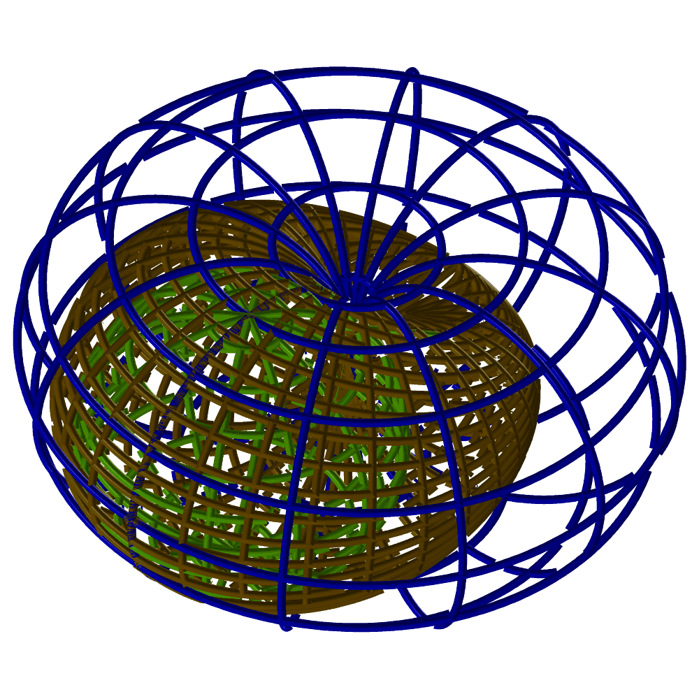
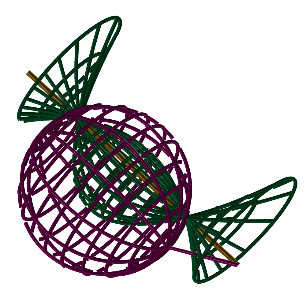
FIGURE: Bisectors of many CSG primitives such as points, lines, planes, spheres, cones, cylinders, and torii are rational. In (left), the rational bisector of a line and a sphere is shown while (right) shows the bisector of a sphere and a torus tangent to each other. See BSCTCONCON, BSCTCONLN, BSCTCONPL, BSCTCONPT, BSCTCONSPR, BSCTCYLPL, BSCTCYLPT, BSCTCYLSPR, BSCTPLNLN, BSCTPLNPT, BSCTSPRLN, BSCTSPRPL, BSCTSPRPT, BSCTSPRSPR, BSCTTRSPT, BSCTTRSSPR, BSCTTRSTRS.
 SurfaceType BSCTTRSTRS( PointType Trs1Pos, VectorType Trs1Dir,
                         NumericType Trs1MjrRad,
                         PointType Trs2Pos, VectorType Trs2Dir,
                         NumericType Trs2MjrRad,
                         NumericType Alpha )
computes the bisector surface between two torii. The torii are located at TrsiPos, with axis of symmetry TrsiDir, a major radius of TrsMajorRad and a minor radius pf TrsMinorRad.
Example:
    BisectSrf = BSCTTRSTRS( point( 0, 0, 0 ), vector ( 0, 0, 1 ), 1,
                            point( -1, 1, 0 ), vector ( 1, 1, 0 ), 1, 0.5 );
See also BSCPCONCON, BSCTCONCN2, BSCTCONCYL, BSCTCONCON, BSCTCONLN, BSCTCONPL, BSCTCONPT, BSCTCONSPR, BSCTCYLPL, BSCTCYLPT, BSCTCYLSPR, BSCTPLNLN, BSCTPLNPT, BSCTSPRLN, BSCTSPRPL, BSCTSPRPT, BSCTSPRSPR, BSCTTRSSPR, CALPHASECTOR, CBISECTOR2D, CBISECTOR3D, SBISECTOR.
BZR2BSP
 CurveType BZR2BSP( CurveType Crv )

 or

 SurfaceType BZR2BSP( SurfaceType Srf )
creates a B-spline curve or a B-spline surface from the given Bezier curve or Bezier surface. The B-spline curve or surface is assigned an open end knot vector(s) with no interior knots, in the parametric domain of zero to one.
Example:
BspSrf = BZR2BSP( BzrSrf );
BSP2BZR
 CurveType | ListType BSP2BZR( CurveType Crv )

 or

 SurfaceType | ListType BSP2BZR( SurfaceType Srf )
creates Bezier curve(s) or surface(s) from a given B-spline curve or a B-spline surface. The B-spline input is subdivided at all internal knots to create Bezier curves or surfaces. Therefore, if the input B-spline does have internal knots, a list of Bezier curves or surfaces is returned. Otherwise, a single Bezier curve or surface is returned. The returned Beziers will have BspDomainMin/Max attributes with the original Bspline domain of the Bezier.
Example:
BzrCirc = BSP2BZR( circle( vector( 0.0, 0.0, 0.0 ), 1.0 ) );
would subdivide the unit circle into four 90 degrees Bezier arcs returned in a list.
C2CONTACT
 CurveType C2CONTACT( CurveType C1, CurveType C2, NumericType StepSizeTol,
                      NumericType SubdivTol, NumericType NumericTol )
computes precise 2-contact planar motion of one curve against the other, building the configuration space of the possible motions. See also "High-Precision Continuous Contact Motion for Planar Freeform Geometric Models", Graphical Model, Vol 76, pp 580-592, 2014, by Yong-Joon Kim, Gershon Elber, and Myung-Soo Kim.}
Example:
MotionPath = C2CONTACT( c1, c2, 1e-3, 1e-3, 1e-8 );
See figure for an example.
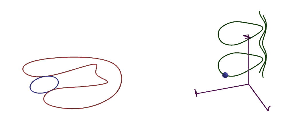
FIGURE: The precise configuration space (three axes for the three degrees of freedom - XY motion and rotation in the plane) is shown on the right for the two curves on the left. The specific configuration on the left is designated as a point on the right. Computed by mapping the contacts formulation into algebraic constraints and solving them.
See also MZERO and MUNIVZERO, MFROMMESH.
CALPHASECTOR
 SurfaceType CALPHASECTOR( ListType TwoCrvs, NumericType Alpha)

 or

 {CurveType | SurfaceType} CALPHASECTOR( ListType CrvPt, NumericType Alpha)
computes the alpha sector for TwoCrvs of E3 type or between a curve and a point, CrvPt. Alpha varies between zero and one. An alpha-sector is created where for Alpha equals zero, the created surface will contain the first curve, and whereas for Tolerance equals one, the created surface will contain the second curve. For CrvPt case, if the Crv is E2, the alpha sector is a curve and if it is E3, the alpha sector is a surface. See also CBISECTOR2D, CBISECTOR3D.
Example:
    c1 = creparam( pcircle( vector( 0.0, 0.0, 0.0 ), 1 ), 0, 1 );
    c2 = cbezier( list( ctlpt( E3, -1.0, 0.0,  1.0 ),
                        ctlpt( E3,  1.0, 0.0, -1.0 ) ) );

    c1 = coerce( c1, E3);
    AlphaSect = CALPHASECTOR( list( c1, c2 ), 0.2 );
    interact( list( c1, c2, AlphaSect ) );
computes the alpha sector surface between the two curves c1 and c2 for alpha equals 0.2.
CANGLEMAP
 CurveType CANGLEMAP( CurveType Crv, NumericType SubdivTol,
                      NumericType Angle, NumericType DiagSpan )

 or

 SurfaceType CANGLEMAP( CurveType Crv, NumericType SubdivTol,
                        NumericType Angle, NumericType DiagSpan )
computes the angular map of planar curve Crv. This bivariate map corresponds pairs of locations in Crv with tangents that are Angle degrees apart. If, for example, Angle is 90 degrees, locations with orthogonal tangents are identified. The zero set of this bivariate map provides the actual correspondence and this zero set is computed with SubdivTol accuracy. If SubdivTol is negative the function whose zero set is the angular map is returned instead. If DiagSpan is non zero, the angular diagonal span is sampled DiagSpan samples and is computed instead. The DiagSpan will provide for each parameter t the forward and backward step that could be taken before hitting an angular span of Angle degrees for the first time.
Example:
    AM = cAngleMap( Crv, 0.01, Angle, false );
    ADS = cAngleMap( Crv, 0.01, Angle, 300 );
computes the Angular map of curve Crv ay angle Angle with subdivison tolerance 0.01 and then extract the angular diagonal span with the same parameters and 300 samples.
See provided figure for more insight. Shown is a given planar curve, with three angular maps of 30, 60 and 90 degrees. The angular diagonal span is also drawn in dark thin lines.
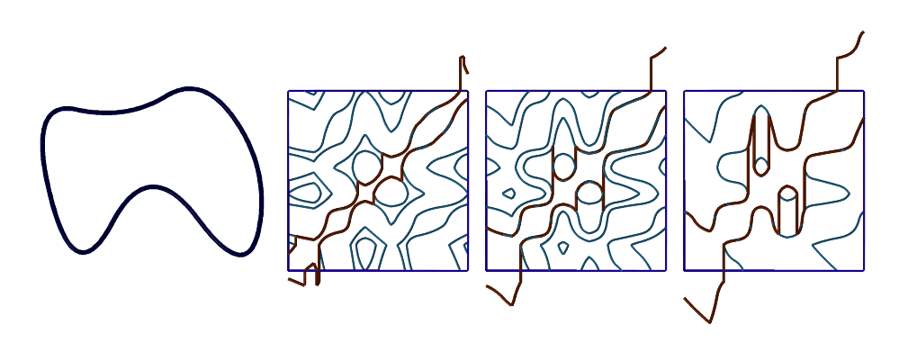
FIGURE: Angular maps computed for the given planar curve on the left, at 30, 60, and 90 degrees, using CANGLEMAP. Also show is the angular diagonal span in thin dark color.
See also CVIEWMAP, CVISIBLE, CARRANGMNT.
CARCLEN
 NumericType CARCLEN( CurveType Crv, NumericType Fineness, NumericType Order )

 or

 CurveType CARCLEN( CurveType Crv, NumericType Fineness, NumericType Order )
Estimates arc length or compute an arc length approximated curve to the given curve. If Order == -1 or 0, the arc length of Crv is computed to within tolerance Fineness, in two different ways. If Order == 2, only the knot vector (if B-spline curve) is adjusted to better reflect and arc-length parameterizations. If Order > 2, approximates an arc length curve out of the given curve Crv. The new approximated curve is sampled with tolerance that is governed by Fineness and will be of order Order. The returned curve is not guaranteed to share the exact same trace as the original curve Crv.
Example:
c2 = carclen( c, 1e-4, 3 );
approximates c as a quadratic arc length curve c2 by sampling the original curve with tolerance 1e-4.
CAREA
CurveType CAREA( CurveType Crv )
computes the integral area curve, ACrv, of the given curve Crv, up to a sign. If Crv is a closed curve with domain t0 to t1, then the difference of ACrv(t1) - ACrv(t0) is the requested area. Example:
    Crv = pcircle( vector( 0, 0, 0 ), 1 );
    ACrv = CAREA( Crv );
    Pi = abs( coord( ceval( ACrv, 4 ), 1 ) - coord( ceval( ACrv, 0 ), 1 ) );
is yet another way of approximating the value of Pi. See also SMOMENTS, SVOLUME and TVOLUME.
CARRANGMNT
 CurveType CARRANGMNT( CurveType Crvs, NumericType Eps,
                       NumericType Operation, PointType CenterPt )
computations over the given arrangment of planar curves Crvs upto accuracy that is governed by Eps. Operation can be one of:
1 - computes all the curve curve intersection locations in the arrangment and keep the results in "InterPts" attributes on the returned curves.
2 - computes all the curve curve intersection locations in the arrangment and split all curves at all those intersections.
3 - computes Y-minimum lower envelop for this curves' arrangement.
4 - computes radial lower envelop around point Center Pt.
CenterPt is ignored if Operation is not equal to 4.
Example:
LinearLowEnv = carrangmnt( Crvs, 1e-12, 3, 0 );
computes the Y-minimum envelop of curve Crvs.
See provided figure for one example of Y-minimum envelop of curves.
FIGURE: Y-minimum envelop for a set of curves, computed using CARRANGMNT. The lower envelop is shown in thick lines.
See also CVIEWMAP, CVISIBLE, CANGLEMAP, CARNGMNT2.
CARNGMNT2
 CurveType CARNGMNT2( CurveType Crvs, NumericType Operation,
                      ListType Params )
computations over the given arrangment of planar curves Crvs upto accuracy. Operation can be one of:
1 - create a new arrangment. Params contains four items: (Tolerance for equality of end points, Planarity tolerance to consider arrangement planar, TRUE to project all curves to be on computed plane, Mask for input type to consider: 0x01 to handle polylines. 0x02 to handle curves. 0x04 to handle trimming curves in trimmed surfaces).
2 - copy an arrangement. Params contains no items.
3 - filter duplications in the input arrangement. Params contains two items: (Epsilon to consider the curves the same, TRUE to update end points to be the same).
4 - filter duplications in the tangential input arrangement. Params contains one item: (Epsilon angle in degrees to consider two curves with the same tangent).
5 - Splits curves at special points, Params contains two items: (Mask for splitting type to consider: 0x01 to split at inflection pts | 0x02 to split at max curvatures | 0x04 to split at C1 disconts, Tolerance of splitting computation).
6 - Split piecewise curves at large angular deviation of adjacent edges. Params contains one item: (Angular deviation (in degrees) to split linear curves at).
7 - Split curves at intersection locations. Params contains one item: (Intersection computation tolerance).
8 - Splits curve near prescribed points. Params contains two items: (A list object of pts to examine and split if near them, Tolerance to consider a point near/on a curve).
9 - Merge adjacent curves. Params contains one item: (Angular deviation (in degrees) to merge C1 discont. curves at).
10 - Least square fit linear curves. Params contains one item: (Fitting Parameter to fit smooth quadratic C1 curves to linear curves. Higher order curves are not affected. If Param positive, the fitted curve size is set to InputCrvSize * FitC1Crv / 100 (i.e. Param serves as percetange of input size). If Param negative, the Fitted curve size is simply set to ABS(Param))
11 - Evaluate the curve arrangement. I.e. loops, hanging edges, etc. Params contains no item.
12 - Classify the curve arrangement. This returns nothing. Params contains no item.
13 - Report the result. Params contains one item: (A mask of desired report: 0x01 to dump info on crvs | 0x02 to also dump the crvs | 0x04 to report end pts in arrangment if evaluated | 0x08 to report regions in arrangment if evaluated).
14 - Dumps to stdout information on the arrangement. Params contains three item: (Style of expected output: 1 for individual crv segs in each region (loop etc.) or 2 for merged curves so every region is one curve or 3 for topology as an ordered list of curve segments and each region is a list of indices into the first list. A negative -i index means index i but a reversed crv. 101, 102, 103: same as 1,2,3 but pt is evaluated at 1/13 of curve parameteric domain to identify orientation, Tolerance of topology reconstruction (in case 3 only), Zoffset in Z for the i'th region, by amount i*ZOffset).
15 - Free a curve arrangement. Params contains no item.
Example:
   ca1 = carngmnt2( crvs2, CA_CREATE, list( 1e-2, 1e-2, TRUE, 7 ) );
   ca2 = carngmnt2( ca1, CA_BREAK_INTER, list( 1e-6 ) );
   ca3 = carngmnt2( ca2, CA_EVAL_CA, list( TRUE ) );
   dm = carngmnt2( ca3, CA_CLASSIFY, nil() );
   CAFinal2 = carngmnt2( ca3, CA_OUTPUT, list( 2, 1e-2, 0.02 ) );
   dm = carngmnt2( ca3, CA_REPORT, list( 1 ) );
   dm = carngmnt2( ca3, CA_REPORT, list( 2 ) );
   dm = carngmnt2( ca3, CA_REPORT, list( 4 ) );
   dm = carngmnt2( ca3, CA_REPORT, list( 8 ) );
Creates a curves' arrangment from crvs2 and classify into closed loops after breaking at all crv-crv intersections.
See also CARRANGMNT.
CBEZIER
CurveType CBEZIER( ListType CtlPtList )
creates a Bezier curve out of the provided control point list. CtlPtList is a list of control points, all of which must be of type (E1-E9 P1-P9), or regular PointType defining the curve's control polygon. The curve's point type will be of a space which is the union of the spaces of all points.
Example:
    s45 = sin(pi / 4);
    Arc90 = CBEZIER( list( ctlpt( P2, 1.0, 0.0, 1.0 ),
                           ctlpt( P2, s45, s45, s45 ),
                           ctlpt( P1, 1.0, 1.0 ) ) );
constructs an arc of 90 degrees as a rational quadratic Bezier curve.
See also CBSPLINE, CPOWER and SBEZIER.
CBIARCS
ListType CBIARCS( CurveType Crv, NumericType Tol, NumericType MaxAngle )
computes bi-arc fitting to a given curve Crv, with a tolarence Tol in L-infinity sense, and a maximum angular span of each arc of at most MaxAngle degrees. Returned is a list of arcs as rational Bezier curves with an arc "center" point attribute to ease the reconstruction of the analytic representation of the geometry.
Example:
  C1 = cbspline( 4,
      list( ctlpt( E3, -0.287, -0.286, 0 ),
            ctlpt( E2, 0.0272, -0.425 ),
            ctlpt( E2, 0.265, -0.0839 ),
            ctlpt( E2, 0.607, -0.165 ),
            ctlpt( E2, 0.832, -0.205 ),
            ctlpt( E2, 0.737, 0.042 ),
            ctlpt( E2, 0.357, 0.103 ),
            ctlpt( E2, 0.508, 0.298 ),
            ctlpt( E2, 0.814, 0.649 ),
            ctlpt( E2, 0.692, 0.775 ),
            ctlpt( E2, 0.411, 0.391 ),
            ctlpt( E2, 0.301, 0.315 ),
            ctlpt( E2, 0.625, 0.945 ),
            ctlpt( E2, 0.49, 1.03 ),
            ctlpt( E2, 0.369, 0.829 ),
            ctlpt( E2, 0.185, 0.384 ),
            ctlpt( E2, 0.194, 0.518 ),
            ctlpt( E2, 0.243, 1.09 ),
            ctlpt( E2, 0.0653, 1.13 ),
            ctlpt( E2, 0.0644, 0.381 ),
            ctlpt( E2, 0.00925, 0.496 ),
            ctlpt( E2, -0.0113, 0.943 ),
            ctlpt( E2, -0.202, 0.954 ),
            ctlpt( E2, -0.147, 0.644 ),
            ctlpt( E2, -0.162, 0.208 ),
            ctlpt( E2, -0.337, -0.156 ) ),
      list( kv_periodic ) );
  C1 = coerce( C1, kv_open );
  Arcs = CBIARCS( Crv, 0.01, 90 );
computes bi-arcs fitting to a given curve in the shape of a human hand, with arcs with at most 90 degrees and tolerance of 0.01. See figure for an example.

FIGURE: Bi-arcs are fitted to the given curve in the shape of a human hand, at two different tolerances, using CBIARCS.
See also QUADCRVS, CUBICCRVS.
CBISECTOR2D
    CurveType  CBISECTOR2D( CurveType Crv,
                            NumericType ZeroSet,
                            NumericType BisectFunc,
                            NumericType Tolerance,
                            NumericType NumerImprove,
                            NumericType SameNormal )

 or

   CurveType   CBISECTOR2D( ListType TwoCrvs,
                            NumericType ZeroSet,
                            NumericType BisectFunc,
                            NumericType Tolerance,
                            NumericType NumerImprove,
                            NumericType SameNormal )

 or

   SurfaceType CBISECTOR2D( ListType CrvPt,
                            NumericType ZeroSet,
                            NumericType UseNrmlTan,
                            NumericType Tolerance,
                            NumericType NumerImprove,
                            NumericType SameNormal )
computes the self bisector curve(s) for Crv or the bisector(s) of TwoCrvs or the bisector of a curve and a point, CrvPt. If ZeroSet is TRUE, the zero-set surface is computed and is used mainly for displaying the zero-set. If it is FALSE, the bisector is returned. The zero-set is computing using the functions F1, F2 and F3 in the paper Gershon Elber and Myung Soo Kim, ``Bisector Curves of Planar Rational Curves,'' CAD, Vol 30, No 14, pp 1089-1096, December 1998} which is determined by the BisectFunc parameter. If BisectFunc = 1, then F1 is used and so on. Tolerance controls the accuracy of the computation, with 0.01 as a good starting value. If Tolerance is negative, NumerImprove can be either TRUE or FALSE, allowing or disabling a final numerical improvement stage. SameNormal can also assume a TRUE or FALSE value, selecting only opposite facing normals, if TRUE. The bisector curve of a curve (E2) and a point CrvPt is computed analytically. Other parameters are ignored. See also CBISECTOR3D, CALPHASECTOR, SBISECTOR.
Example:
    c1 = cbezier( list( ctlpt( E2, -0.5, -0.2 ),
                        ctlpt( E2,  0.0, -0.2 ),
                        ctlpt( E2,  0.6,  0.6 ) ) );
    c2 = cbezier( list( ctlpt( E2,  0.3, -0.7 ),
                        ctlpt( E2, -0.2, -0.7 ),
                        ctlpt( E2,  0.7,  0.6 ) ) );
    BisectCrvs = CBISECTOR2D( list( c1, c2 ), TRUE, 1, 0.01, true, false );
    All = list( c1, c2, BisectCrvs );
    interact( list( All, view_mat2d ) );
computes the bisector for planar curves as a set of bisector curves. See figure for an example.
CBISECTOR3D
 SurfaceType CBISECTOR3D( ListType TwoCrvs, NumericType BisectFunc)

 or

 SurfaceType CBISECTOR3D( ListType CrvPt, NumericType BisectFunc)

 or

 SurfaceType CBISECTOR3D( ListType TwoCrvsSrf, NumericType BisectFunc)

 or

 SurfaceType CBISECTOR3D( ListType CrvPtSrf, NumericType BisectFunc)
computes the bisector surface TwoCrvs or the bisector surface of a curve and a point, CrvPt, in R3. The BisectFunc determines the function to be used for generating the bisector surface between the two E3 curves. If 1, a 3-space bisector surface is generated to the given curves or a curve and a point. If 4, a surface whose zero set prescribes the bisectors of the given curves is returned. if 2, and a surface is also attached to the list (last two option above) the geometry (curves/point) is assume in the domain of the surface and the bisector curve is computed in the surface. See also CBISECTOR2D, CALPHASECTOR, SBISECTOR.
Example:
    c1 = creparam( pcircle( vector( 0.0, 0.0, 0.0 ), 1 ), 0, 1 );
    c2 = cbezier( list( ctlpt( E3, -1.0, 0.0,  1.0 ),
                        ctlpt( E3,  1.0, 0.0, -1.0 ) ) );
    c1 = coerce( c1, E3);
    BisectSrf = CBISECTOR3D( list( c1, c2 ), 1 );
    interact( list( c1, c2, BisectSrf ) );
computes a bisector surface of a Z parallel line and a circle in the XY plane. See figure for an example.
FIGURE: (left) Bisectors of two quadratic Bezier curves in the plane. (right) A bisector surface of a line and a circle in three space. See the CBISECTOR2D and CBISECTOR3D functions respectively.
CBSPLINE
 CurveType CBSPLINE( NumericType Order, ListType CtlPtList,
                                                        ListType KnotVector )
creates a B-spline curve out of the provided control point list, the knot vector, and the specified order. CtlPtList is a list of control points, all of which must be of type (E1-E9 P1-P9, or regular PointType defining the curve's control polygon. The curve's point type will be of a space which is the union of the spaces of all points. The length of the KnotVector must be equal to the number of control points in CtlPtList plus the Order. If, however, the length of the knot vector is equal to #CtlPtList + Order + Order - 1, the curve is assumed to be periodic. The knot vector list may be specified as either list( KV_OPEN ), list( KV_FLOAT ) or list( KV_PERIODIC ) in which a uniform open, uniform floating or uniform periodic knot vector with the appropriate length is automatically constructed.
Example:
    s45 = sin(pi / 4);
    HalfCirc = CBSPLINE( 3,
                         list( ctlpt( P3,  1.0,  1.0,  0.0, 0.0 ),
                               ctlpt( P3,  s45,  s45,  s45, 0.0 ),
                               ctlpt( P3,  1.0,  0.0,  1.0, 0.0 ),
                               ctlpt( P3,  s45, -s45,  s45, 0.0 ),
                               ctlpt( P3,  1.0, -1.0,  0.0, 0.0 ) ),
                         list( 0, 0, 0, 1, 1, 2, 2, 2 ) );
constructs an arc of 180 degrees in the XZ plane as a rational quadratic B-spline curve.
Example:
    c = CBSPLINE( 4,
                  list( ctlpt( E2,  0.5,  0.5 ),
                        ctlpt( E2, -0.5,  0.5 ),
                        ctlpt( E2, -0.5, -0.5 ),
                        ctlpt( E2,  0.5, -0.5 ) ),
                  list( KV_PERIODIC ) );
    color( c, red );
    viewobj( c );

    c1 = cregion( c, 3, 4 );
    color( c1, green );
    c2 = cregion( c, 4, 5 );
    color( c2, yellow );
    c3 = cregion( c, 5, 6 );
    color( c3, cyan );
    c4 = cregion( c, 6, 7 );
    color( c3, magenta );
    viewobj( list( c1, c2, c3, c4 ) );
creates a periodic curve and extracts its four polynomial domains as four open end B-spline curves. See figure for an example.
FIGURE: A cubic periodic curve created using KV_PERIODIC end conditions.
See also CBEZIER, CPOWER and SBSPLINE.
CCINTER
 ListType CCINTER( CurveType Crv1, CurveType Crv2, NumericType Epsilon,
                                                       NumericType SelfInter )

 or

 SurfaceType CCINTER( CurveType Crv1, CurveType Crv2, NumericType Epsilon,
                                                       NumericType SelfInter )
compute the intersection point(s) of Crv1 and Crv2 in the XY plane. Since this computation involves numeric operations, Epsilon controls the accuracy of the parametric values of the result. It returns a list of PointTypes, each containing the parameter of Crv1 in the X coordinate, and the parameter of Crv2 in the Y coordinate. If, however, Epsilon is negative, a scalar field surface representing the square of the distance function is returned instead. If SelfInter is TRUE, Crv1 and Crv2 can be the same curve, and self intersection points are searched for instead.
Example:
 crv1 = cbspline( 3,
                  list( ctlpt( E2, 0, 0 ),
                        ctlpt( E2, 0, 0.5 ),
                        ctlpt( E2, 0.5, 0.7 ),
                        ctlpt( E2, 1, 1 ) ),
                  list( KV_OPEN ) );
 crv2 = cbspline( 3,
                  list( ctlpt( E2, 1, 0 ),
                        ctlpt( E2, 0.7, 0.25 ),
                        ctlpt( E2, 0.3, 0.5 ),
                        ctlpt( E2, 0, 1 ) ),
                  list( KV_OPEN ) );
 inter_pts = CCINTER( crv1, crv2, 0.0001, FALSE );
computes the parameter values of the intersection point of crv1 and crv2 to a tolerance of 0.0001. See figure for an example.
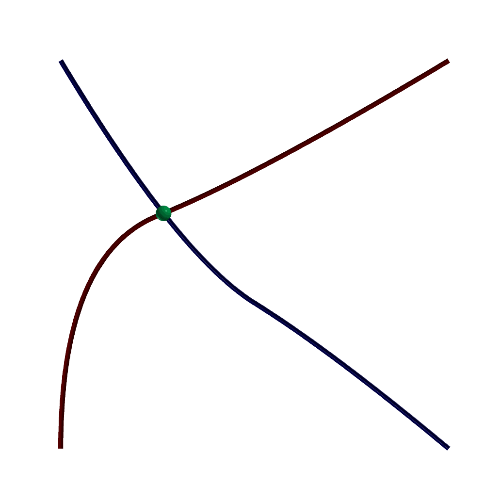
FIGURE: A intersection point of two freeform curve computed using CCINTER.
CCRVTR
 ListType CCRVTR( CurveType Crv, NumericType Epsilon, NumericType Operation )

 or

 CurveType CCRVTR( CurveType Crv, NumericType Epsilon, NumericType Operation )
computes the curvature field's magnitude square of Crv in the XY plane if Operation is 1, or its extreme points if Operation equals 2. This set includes not only points of maximum (convexity) and mimumum (concavity) curvature, but also points of zero curvature locations, such as inflection points. A list of parameter value(s) of the location(s) with extreme curvature along the Crv is returned in the latter case. Since this operation is partially numeric, Epsilon is used to set the needed accuracy. If, however, Operation is 3, the input curve is being split at the extreme curvature location and a list of curve segments is returned instead.
This function computes the (square of the) curvature scalar field for
planar curves as,
x' y'' - x'' y'
k(t) = ----------------
2 2 3/2
( x' + y' )
and computes (the square of) kN for three-dimensional curves as the
following vector field,
C' x C'' C' (C' x C'') x C'
k(t) N(t) = K(t) B(t) x T(t) = -------- x ----- = ---------------
3 | C' | 4
| C'| | C' |The extremum values are extracted from the computed curvature field. This (square of the) curvature field is a high order curve, even if the input geometry is of low order. This is especially true for rational curves, for which the quotient rule for differentiation is used and almost doubles the degree in every differentiation.
See also CCRVTREVAL, CINFLECT, CNRMLCRV, CZEROS, CEXTREMES, and SCRVTR.
Example:
 crv = cbezier( list( ctlpt( E2, -1.0,  0.5 ),
                      ctlpt( E2, -0.5, -2.0 ),
                      ctlpt( E2,  0.0,  1.0 ),
                      ctlpt( E2,  1.0,  0.0 ) ) ) * rotz( 30 );
 crvtr = CCRVTR( crv, 0.001, 2 );
 pt_crvtr = nil();
 pt = nil();
 for ( i = 1, 1, sizeof( crvtr ),
     ( pt = ceval( crv, nth( crvtr, i ) ) ):
     snoc( pt, pt_crvtr )
 );
 interact( list( crv, pt_crvtr ) );
finds the extreme curvature points in Crv and displays them all with the curve. See figure for an example.
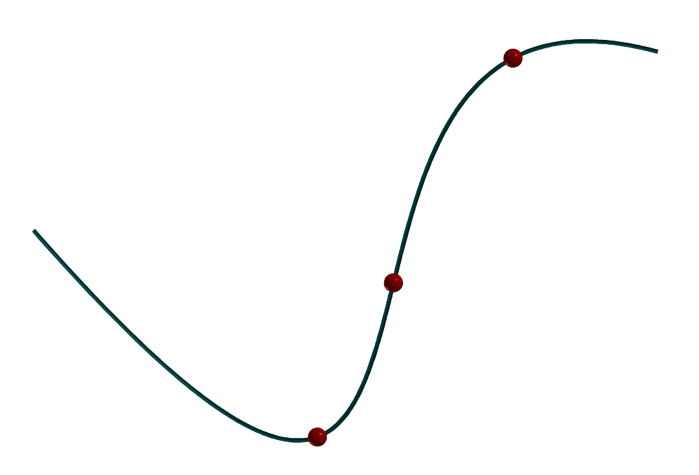
FIGURE: Extreme curvature locations on a freeform curve computed using CCRVTR.
CCRVTR
 PolyType CCRVTR1PT( CurveType Crv, NumericType CtlPtIdx, NumericType Min,
                     NumericType Max, NumericType SubdivTol, NumericType NumerTol,
                     NumericType Operation )

 or

 MultivarType CCRVTR1PT( CurveType Crv, NumericType CtlPtIdx, NumericType Min,
                     NumericType Max, NumericType SubdivTol, NumericType NumerTol,
                     NumericType Operation )
computes the topology changes in the curvature field of curve Crv as control point index CtlPtIdx in the curve is moving. The motion of the control points is limited to be between Min and Max in X and Y. See MZERO for the meaning of the SubdivTol and NumerTol. The returned value depends on Operation: If Operation is 0, a multivariate of dim(Crv) + 1 that is representing the curvature topology field is returned. If Operation is 1, the marching cubes of Operation == 0 is computed and returned as a polygonal surface. If Operation is 2 the silhouette of 1 is computed and returned and if Operation is 3 the result of 2 is evaluated back into Euclidean space.
Example:
MV = CCRVTR1PT( Crv, 4, Min, Max, 0.01, 1e-10, 1 );
CCRVTREVAL
NumericType CCRVTREVAL( CurveType Curve, NumericType t )
computes the curvature of curve Curve at parameter t.
Example:
k = CCRVTREVAL(Crv, 0.5 );
See also CCRVTR.
CCUBICS
CurveType CCUBICS( CurveType Crv, NumericType Tolerance )
returns a list of cubic curves approximating the given curve Crv to within Tolerance.
Example:
Crv = CCUBICS( Crv, 0.01 );
See figure for an example.
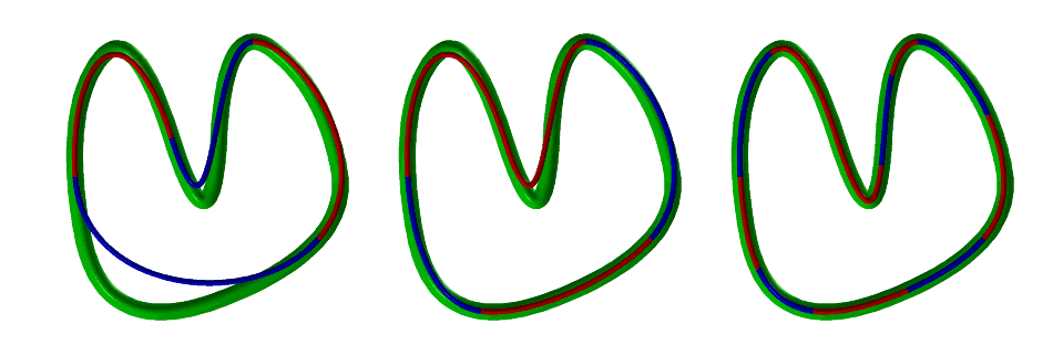
FIGURE: A piecewise cubic fit to a given general curve, at three different tolerances, using CCUBICS.
See also CUBICCRVS, QUADCRVS, and CBIARCS.
CDERIVE
CurveType CDERIVE( CurveType Curve )
returns a vector field curve representing the differentiated curve, also known as the Hodograph curve.
Example:
 Circ = circle( vector( 0.0, 0.0, 0.0 ), 1.0 );
 Hodograph = CDERIVE( Circ );
See figure for an example.
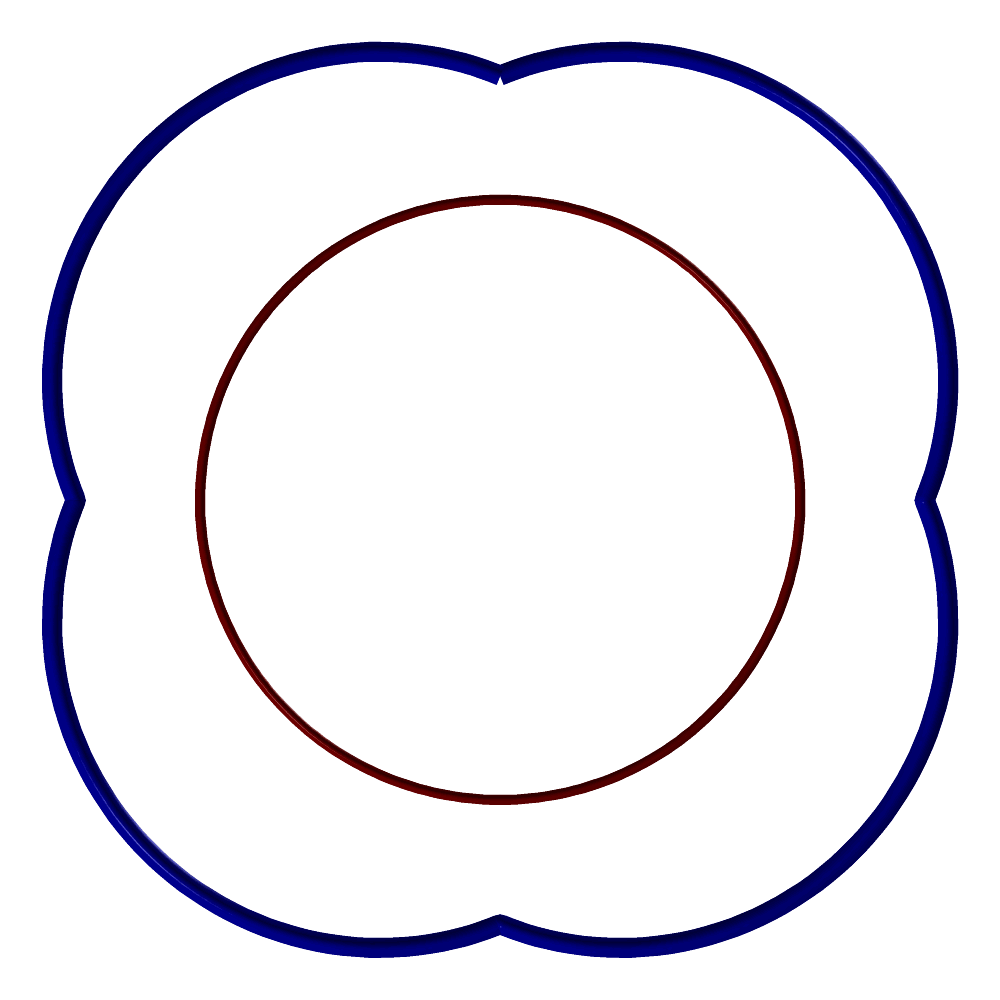
FIGURE: The Hodograph (thick) of a B-spline circle (thin) constructed as four 90 degrees rational Bezier arcs, computed using CDERIVE.
See also CINTEG, SDERIVE, TDERIVE, and MDERIVE
CDIVIDE
ListType CDIVIDE( CurveType Curve, NumericType Param )
subdivides a curve into two sub-curves at the specified parameter value. Curve can be either a B-spline curve in which Param must be within the Curve's parametric domain, or a Bezier curve in which Param can be arbitrary, extrapolating if not in the range of zero to one.
It returns a list of the two sub-curves. The individual curves may be extracted from the list using the NTH command.
Example:
 CrvLst = CDIVIDE( Crv, 1.3 );
 Crv1 = nth( CrvLst, 1 );
 Crv2 = nth( CrvLst, 2 );
subdivides the curve Crv at the parameter value of 0.5. See figure for an example.
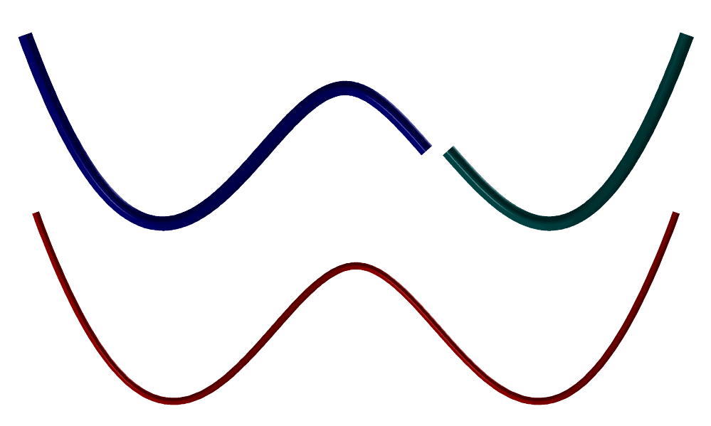
FIGURE: A B-spline curve is subdivided into two distinct regions using CDIVIDE.
See also SDIVIDE, TDIVIDE, and MDIVIDE
CEDITPT
CurveType CEDITPT( CurveType Curve, CtlPtType CtlPt, NumericType Index )
provides a simple mechanism to manually modify a single control point number Index (base count is 0) in the Curve, by substituting CtlPt instead. CtlPt must have the same point type as the control points of the Curve. If, however, CtlPt is not a control point object, control point number Index is deletedfrom the input curve. The original curve Curve is not modified.
Example:
    CPt = ctlpt( E3, 1, 2, 3 );
    NewCrv = CEDITPT( Curve, CPt, 1 );
constructs a NewCrv with the second control point of Curve being CPt.
CENVOFF
 SurfaceType CENVOFF( CurveType Curve,
                      NumericType Height, NumericType Tolerance )

 or

 ListType CENVOFF( CurveType Curve, NumericType Height, NumericType Tolerance )
computes the offset envelope of a given planar curve Curve. The offset envelope is the envelope of cones with apex on point on Curve in the Z direction. Height is the height of the cone which also equals the offset distance or the width of the cones. Tolerance controls the accuracy of the offset approximation.
If the Curve is closed, two surfaces are created in the offset envelope, one for the inside and another for the outside. If Curve is open, a single envelope offset surface is computed, wrapping around both sides.
Example:
    c1 = cbezier( list( ctlpt( E2, -0.8, 0.0 ),
                        ctlpt( E2, -0.2, 1.0 ),
                        ctlpt( E2,  0.2, 0.0 ),
                        ctlpt( E2,  0.8, 0.6 ) ) );
    s1 = CENVOFF( c1, 0.5, 0.01 );
computes an envelope offset surface for a cubic Bezier curve c1 of Height of 0.5 and Tolerance of 0.01. See figure for an example.
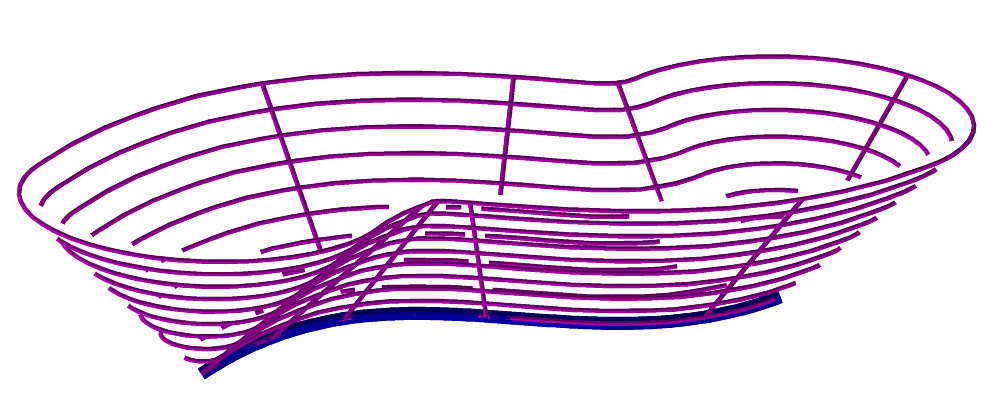
FIGURE: The envelope offset of a freeform planar curve computed using CENVOFF.
CEVAL
CtlPtType CEVAL( CurveType Curve, NumericType Param )
evaluates the provided Curve at the given Param value. Param should be in the curve's parametric domain if the Curve is a B-spline curve, or between zero and one if the Curve is a Bezier curve. The returned control point has the same point type as the control points of the Curve.
Example:
CPt = CEVAL( Crv, 0.25 );
evaluates Crv at the parameter value of 0.25. See also SEVAL, MEVAL, TEVAL.
CEXTREMES
ListType CEXTREMES( CurveType Crv, NumericType Epsilon, NumericType Axis )
computes the extreme set of the given Crv in the given axis (1 for X, 2 for Y, 3 for Z). Since this computation is numeric, an Epsilon is also required to specify the desired tolerance. It returns a list of all the parameter values (NumericType) in which the curve takes an extreme value.
Example:
extremes = CEXTREMES( Crv, 0.0001, 1 );
computes the extreme set of curve crv, in the X axis, with error tolerance of 0.0001. See also CZERO. See figure for an example.
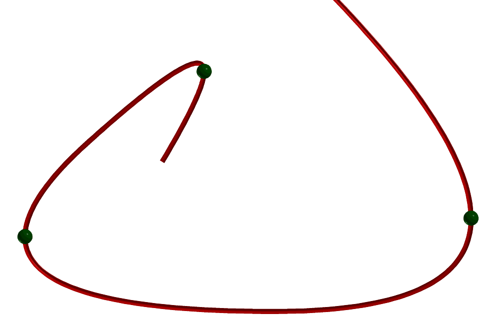
FIGURE: The X local extremums of a freeform curve are isolated using CEXTREMES.
CFNCRVTR
 CurveType CFNCRVTR( CurveType E2Crv, NumericType Samples,
                     NumericType Order, NumericType ArcLen )

 or

 CurveType CFNCRVTR( CurveType CrvtrE1Crv, NumericType Accuracy,
                     NumericType Order, NumericType Periodic )
computes the curvature field of planar curve E2Crv in the first form, and reconstructs an E2 planar curve from the given curvature field CrvtrE1Crv in the second form. In the first form, Samples defines the numer of samples to use along the input curve while if ArcLen TRUE the samples are also made along the arc length of E2Crv. In the second form, a planar curve is reconstructed from the curvature field of CrvtrE1Crv, with Accuracy to control the accuracy. If the reconstructed curve is suppose to be closed, set Periodic to TRUE. In both forms, Order sets the order of the return curve.
Example:
CrvtrField = CFNCRVTR( Crv, 1000, 2, TRUE );
CHELIX
 CurveType CHELIX( NumericType NumLoops, NumericType Pitch,
                   NumericType Radius, NumericType Samples,
                   NumericType CtlPtsPerLoop )
constructs a polynomial approximation of a helical curve of NumLoops loops and specified Radius and Pitch. The curve is approximated as a least sqaures fit of Samples samples and CtlPtsPerLoop control points per loop.
Example:
HelixcalCrv = chelix( 3, 0.333, 0.444, 100, 6 );
See figure for this helix of 3 loops.
FIGURE: Approximates a helical curve using CHELIX.
See also CSPIRAL, CSIN
CIEXTREME
 ListType CIEXTREME( SurfaceType Srf, NumericType Dir,
                     NumericType SubdivTol, NumericType NumerTol )
computes the X- or Y-extreme values of the implicit univariate defined as the zero set of Srf. In addition, this function also detects hyperbolic tangent contact of Srf with the plane Z = 0. Dir specified the desired direction of the extremum to extract, one of COL or ROW. See MZERO for the meaning of the SubdivTol and NumerTol.
Example:
ViewMap = CIEXTREME( Srf, col, 0.01, 1e-9 );
See figure for an example.
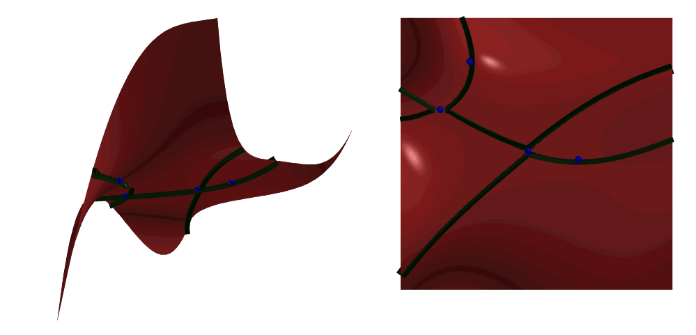
FIGURE: An example of computing the X- and Y-extreme locations of this implicit curve defined as the zero set of the surface. Also detected surface tangency contacts with the plane Z = 0.
CINFLECT
 ListType CINFLECT( CurveType Crv, NumericType Epsilon, NumericType Operation )

 or

 CurveType CINFLECT( CurveType Crv, NumericType Epsilon,
                     NumericType Operation )
computes and returns a scalar field (the numerator of the curvature field, the sign of the curvature field if you like) whose zeros are the inflection points of Crv in the XY plane, if Operation is 1. If Operation is 2, the inflection points are derived and returned as list of all the parameter values (NumericType) in which the curve has an inflection point. Since this computation is partially numeric, an Epsilon is also required to specify the desired tolerance. If, however, Operation is 3, the input curve Crv is being split at all the inflection points and the different, inflection free, curve segements are returned in a list.
The sign of curvature scalar field is equal to
s(t) = x' y'' - x'' y'Example:
    inflect = CINFLECT( crv, 0.001, 2 );
    pt_inflect = nil();
    pt = nil();
    for ( i = 1, 1, sizeof( inflect ),
            pt = ceval( crv, nth( inflect, i ) ):
            snoc( pt, pt_inflect )
        );
    interact( list( axes, crv, pt_inflect ) );
computes the set of inflection points of curve crv with error tolerance of 0.001. This set is then scanned in a loop and evaluated to the curve's locations which are then displayed with the crv. See also CZEROS, CEXTREMES, and CCRVTR. See figure for an example.
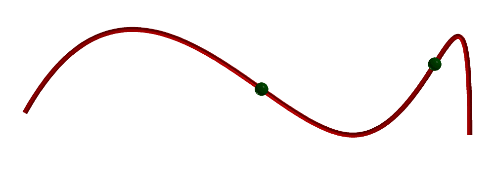
FIGURE: The Inflection points of a freeform curve can be isolated using CINFLECT.
CINTEG
CurveType CINTEG( CurveType Crv );
returns a vector field curve representing the integral curve. See also CDERIVE.
CINTERP
 CurveType CINTERP( ListType PtList, NumericType Order, NumericType Tol,
        NumericType C1Discont, NumericType Periodic, NumericType EndPtInterp )

 or

 CurveType CINTERP( ListType PtList, NumericType Order, NumericType Size,
          ConstantType Params, NumericType Periodic, NumericType EndPtInterp )

 or

 CurveType CINTERP( CurveType Crv, NumericType Order, NumericType Size,
              ListType Params, NumericType Periodic, NumericType EndPtInterp )
computes a B-spline curve that interpolates or approximates the list of (control) points in PtList or a given curve Crv. The B-spline curve will have order Order and either Size control points (if integer) or automatically computed Tol (if is/has a fraction) in L-infinity norm of the deviation of the curve from the given list of (control) points. If Tol is used, C1Discont sets the cosine of the maximal angle to consider as C^1 discontinuity (or -1 to disable). The created curve will be periodic if periodic is non zero. The knots will be spaced according to Param which can be one of PARAM_UNIFORM, PARAM_CHORD, PARAM_CENTRIP, PARAM_NEILFOL, or lists of parameter values and knots (see below). The PARAM_UNIFORM prescribes a uniform knot sequence, PARAM_CHORD specifies knot spacing according to the chord length and PARAM_CENTRIP according to the square root of the chord length. Finally, PARAM_NEILFOL takes into consideration the angles between three consecutive points. A periodic curve will be coerced to have a PARAM_UNIFORM knot sequence. If Params is a list object, it should contain preciely two item: 1. The first item is typically a list containing the parameter values at which to approximate or interpolate the data points. Hence, the length of this list must equal the length of the PtList data. However, this item can also be either PARAM_UNIFORM or PARAM_CHORD for parameters to be automatically set unitformally or at chord length. 2. The second item is a list specifies the knot vector of the construct B-spline curve. Use of Periodic end conditions can create cases with degenerated linear systems (determinant equal zero). Increase or decrease of the Order of the B-spline by one might resolve the problem. All points in PtList must be of type (E1-E9, P1-P9) control point, or regular PointType. If Size is equal to the number of points in PtList, the resulting curve will interpolate the data set. Otherwise, if Size is less than the number of points in PtList, the point data set will be least square approximated. At no time can Size be lower than Order. Size of zero forces interpolation by selecting Size to be the size of the data set. If EndPtInterp TRUE, then the end points of the fitted curve will interpolate the first and last point in PtList. All interior knots will be distinct, preserving maximal continuity.
Example:
    pl = nil();
    for ( x = 0, 1, 100,
          snoc(point(cos(x / 5), sin(x / 5), x / 50 - 1), pl)
    );
    attrib( nref( pl, 1 ), "C0Bndry", true );
    c = CINTERP( pl, 3, 21, PARAM_UNIFORM, false, false );
samples a helical curve at 100 points and least square fit of a quadratic B-spline curve with 21 points to the data set. The curve will have a uniform knot spacing and is not periodic. See also figure for an example. Another example, having pl as a list of 11 points:
 c2 = cinterp( pl, 3, 11,
               list( list( 0.0, 0.1, 0.2, 0.3, 0.4, 0.5,
                           0.6, 0.7, 0.8, 0.9, 1 ),
                     list( 0.0, 0.0, 0.0, 0.1, 0.2, 0.4, 0.4,
                           0.6, 0.6, 0.8, 0.9, 1.0, 1.0, 1.0 ) ),
               0, 1 );
interpolates the points in pl while using the sepcified knot vector and interpolaion parameters. See also SINTERP, TINTERP and LINTERP.
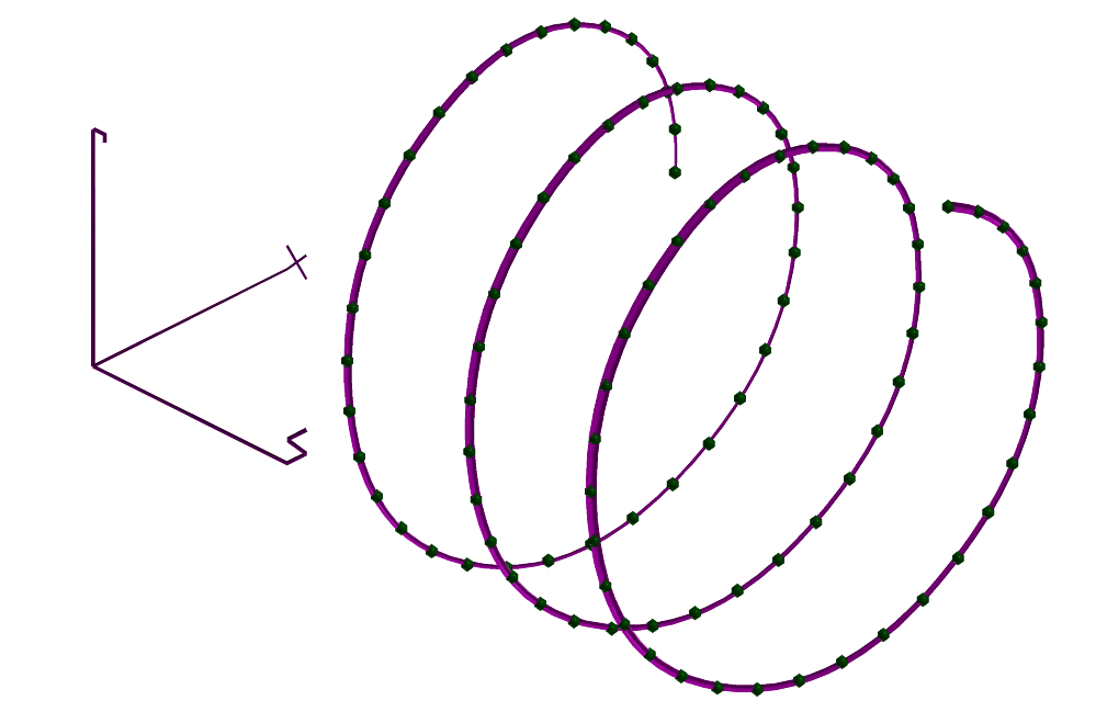
FIGURE: A Helix, sampled at 100 locations, is least square fitted using CINTERP by a quadratic B-spline curve and 21 control points.
See also CINTERP2.
CINTERP2
CurveType CINTERP2( CurveType Crv, NumericType InflectStretch )
Computes a quadratic interpolating curve to the control polygon of the given curve Crv, directly. No linear system is created/solved and the interpolation is ensured by adjusting the spacings between knots. InflectStretch afftects the way inflection locations in Crv are affected. A value of 1.0 is a good start for InflectStretch.
Example:
    c = cbspline( 2,
                  list( point( 0, 0, 0 ),
                        point( 1, 0, 0 ),
                        point( 1, 1, 0 ),
                        point( 2, 1, 0 ) ),
                  list( kv_open ) );
    ci1 = CINTERP2( c, 1.0 );
    ci2 = CINTERP2( c, 0.5 );
    ci3 = CINTERP2( c, 0.25 );
Fits three quadratic B-spline curves, Cij, through the control polygon of Crv, with different inflection location tension.
See also CINTERP.
CIRCLE
CurveType CIRCLE( VectorType Center, NumericType Radius )
constructs a circle at the specified Center with the specified Radius. The returned circle is a B-spline curve of four piecewise Bezier 90 degree arcs. The construced circle is always parallel to the XY plane. Use the linear transformation routines to place the circle in the appropriate orientation and location.
CIRCPACK
 CurveType CIRCPACK( CurveType Boundary,
                     NumericType Radius,
                     NumericType NumIter,
                     NumericType NumerTol,
                     NumericType SubdivTol )
Computes a dense packing of circles of Radius inside a two dimensional container specified by its Boundary. A perturbation approach is adopted which simulates shaking of container under gravity. NumIter specifies the maximum iterations to elapse without making progress. The numeric tolernace and subdivision tolerances are specified by NumerTol and SubdivTol, respectively. The function returns a list of circles.
Example:
circlelist = CIRCPACK( C, 0.06, 15, 1e-9, 5e-2 );
See figure for an example.
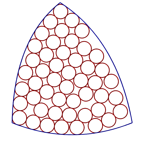
FIGURE: A dense packing of circles inside a freeform container, using CIRCPACK.
CIRCPOLY
PolygonType CIRCPOLY( VectorType Normal, VectorType Trans, NumericType Radius )
defines a circular polygon in a plane perpendicular to Normal that contains the Trans point. The constructed polygon is centered at Trans. RESOLUTION vertices will be defined with Radius from distance from Trans.
Alternative ways to construct a polygon are manual construction of the vertices using POLY, or the construction of a flat ruled surface using RULEDSRF.
CLNTCRSR
ListType CLNTCRSR( NumericType TimeOut )
reads the mouse coordinates as well as mouse events from displace devices, or times out after TimeOut miliseconds. A list object of two sub-objects, a points and a vector, named "_PickCrsr_" is returned. These point and vector define the three-dimensional line of the mouse in object space.
Mouse events are typically processed by the display device. However, by the command "CLNTPICKCRSR" (in iritinit.irt) which sends a "PICKCRSR" request to the display devices, mouse events will be sent to the server. The server can be requested to keep mouse events for "CLNTCRSR" to be read via the IritState command and the "CursorKeep" attribute.
Both the point and the vector will have a numeric attribute of "EventType" that will have the following meaning:
| 1 | Mouse motion event |
|---|---|
| 2 | Mouse down event |
| 5 | Mouse up event |
Example:
   ClntPickCrsr( clients_all );

   IritState( "CursorKeep", 1 );

   Quit = 0;
   for ( i = 0, 1, 10,
       CLNTCRSR( 10000 ) );

   ClntPickDone( clients_all );
   IritState( "CursorKeep", 0 );
asks all clients to send mouse events to the server, asks the server to keep mouse events, and then reads 10 mouse events.
CLNTREAD
AnyType CLNTREAD( NumericType Handler, NumericType Block )
reads one object from a client communication channel. Handler contains the index of the communication channel opened via CLNTEXEC. If no data is available in the communication channel, this function will block for at most Block milliseconds until data is found or timeout occurs. In the latter, a single StringType object is returned with the content of "no data (timeout)". If Handler equals -1, the regular display device (forked via, for example, VIEWOBJ command) is used. See also VIEWSET, CLNTWRITE, CLNTCLOSE, and CLNTEXEC.
Example:
   h2 = clntexec( "xmtdrvs -s-" );
       .
       .

   Model = CLNTREAD( h2 );
       .
       .

   clntclose( h2,TRUE );
reads one object from client through communication channel h2 and saves it in variable model.
CMAT2D
CurveType CMAT2D( CurveType Crv, NumericType SubdivTOl, NumericType NumerTol )
computes the medial axis transform of a give closed palanar curve Crv. Not supported.
Example:
MAT = CMAT2D( Crv, 1e-3, 1e-10 );
CMESH
CurveType CMESH( SurfaceType Srf, ConstantType Direction, NumericType Index )
returns a single ROW or COLumn as specified by the Direction and Index (base count is 0) of the control mesh of surface Srf.
The returned curve will have the same knot vector as Srf in the appropriate direction. See also CSURFACE.
This curve is not necessarily in the surface Srf.
Example:
Crv = CMESH( Srf, COL, 0 );
extracts the first column of surface Srf as a curve. See also CSURFACE. See also SMESH, MFROMMESH.
CMOEBIUS
CurveType CMOEBIUS( CurveType Crv, NumericType Ratio )
rebalances the weights of a rational curve using the Moebius transformation. The shape of the curve remains identical while the speed is modified. Ratio controls the ratio between the last and the first weights. If Ratio = 0, the first and last weights are made equal.
See also SMOEBIUS.
CMORPH
 CurveType CMORPH( CurveType Crv1, CurveType Crv2,
                   NumericType Method, NumericType Blend )

 or

 ListType CMORPH( CurveType Crv1, CurveType Crv2,
                  NumericType Method, NumericType Blend )
create a new curve which is a metamorph of the two given curves. The two given curves must be compatible (see FFCOMPAT) before this blend is invoked. This is very useful if a sequence that "morphs" one curve to another is to be created. Several metamorphosis methods are supported according to the value of Method,
| 0 | Simple convex blend. |
|---|---|
| 1 | Corner/Edge cutting scheme, scaled to same curve length. |
| 2 | Corner/Edge cutting scheme, scaled to same bounding box. |
| 3 | Same as 1 but with filtering out of tangencies. |
| 4 | Same as 2 but with filtering out of tangencies. |
| 5 | Multiresolution decomposition based metamorphosis. See CMULTRES. |
In Methods 2 to 5, Blend is a step size for the metamorphosis operation and a whole list describing the entire metamorphosis operation is returned.
Examples:
    for ( i = 0, 1, 300,
        c = CMORPH( crv1a, crv1b, 0, i / 300.0 ):
        color( c, yellow ):
        viewobj( c )
    );

    crvs = CMORPH( crv1a, crv1b, 2, 0.003 );
    snoc( crv1b, crvs );
    for ( i = 1, 1, sizeof( crvs ),
        c = nth( crvs, i ):
        color( c, yellow ):
        viewobj( c )
    );

    Turtle2 = ffmatch( Wolf, Turtle, 20, 100, 2, false, 2 );
    ffcompat( Wolf, Turtle2 );
    for ( i = 0, 1, 25,
        c = CMORPH( Wolf, Turtle2, 0, i / 25 ):
        color( c, yellow ):
        viewobj( c )
    );
creates three metamorphosis animation sequences, one that is based on a convex blend, and two that are based on corner/edge cutting schemes. See also PMORPH, SMORPH, TMORPH, and FFMATCH. See figure for an example.
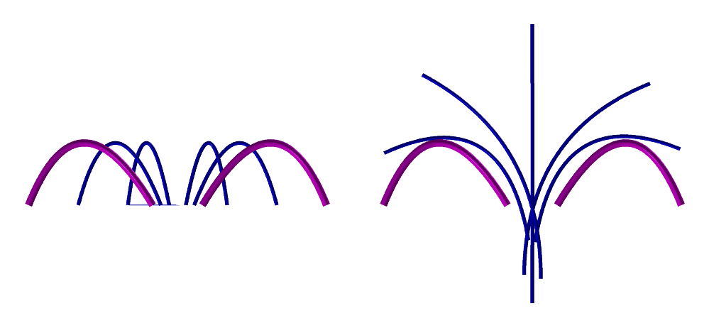
FIGURE: A morphing sequence using convex blend (top left), edge cutting (top right), and using FFMATCH and convex blend (bottom).
CMULTIRES
 ListType CMULTIRES( CurveType Crv, NumericType Discont,
                                                NumericType LeastSquares )
computes a multiresolution decomposition of curve Crv using least squares approximation, if LeastSquares is TRUE, or using B-Wavelets if LeastSquares is FALSE. The latter is optimal but slower. The resulting list of curves describes an hierarchy of curves in linear subspaces of the space in which Crv lay. If LeastSquares is TRUE, the curves could be summed algebraically to form Crv. Each of the curves in the hierarchy is a least squares approximation of Crv in the subspace in which it is defined. If LeastSquares is FALSE, a list of orthogonal projections of the Crv onto the prescibed subspaces (by the knot sequences) is provided. Finally, Discont is a Boolean flag that controls the way tangent discontinuities are preserved throughout the decomposition. If, however, Discont is -1, LeastSquares will indicate the index of the knot in Crv to compute its BWavelet function.
Example:
    MRCrv = CMULTIRES( Animal, false, true );

    sum = nth( MRCrv, 1 );
    MRCrvs = list( sum * tx( 3.0 ) );
    for ( ( i = 2 ), 1, sizeof( MRCrv ),
        sum = symbsum( sum, nth( MRCrv, i ) ):
        snoc( sum * tx( ( 3 - i ) * 1.5 ), MRCrvs )
    );

    All = MRCrvs * sc ( 0.25 );
    view( All, on );
computes a multiresolution decomposition to curve CrossSec as MRCrv and displays all the decomposition levels by summing them all up. The use of none as on object name allows one to display an object in the display device without replacing the previous object in the display device, carrying the same name.
This creates two metamorphosis animation sequences, one based on a convex blend and one based on a corner/edge cutting scheme. See figure for an example.
FIGURE: A multiresolution decomposition of a curve of an animal using least squares. The original curve is shown on the left.
CNORMAL
VectorType CNORMAL( CurveType Crv, NumericType TParam )
computes the normal vector to curve Crv at the parameter values TParam. The returned vector has a unit length.
Example:
Normal = CNORMAL( Crv, 0.5 );
computes the normal to Crv at the parameter value 0.5. See also CNRMLCRV, CTANGENT.
CNRMLCRV
CurveType CNRMLCRV( CurveType Crv )
symbolically computes a vector field curve representing the non-normalized normals of the given curve. That is, a normal vector field, evaluated at t, provides a vector in the direction of the normal of the original curve at t. The normal curve once computed is in fact equal to kN where k is the curvature of Crv and N is its normal.
Example:
NrmlCrv = CNRMLCRV( Crv );
See also CCRVTR.
CNVXHULL
 PolygonType CNVXHULL( PolygonType Poly | PolylineType Poly,
                       NumericType FineNess );

 or

 CurveType CNVXHULL( CurveType Crv, NumericType FineNess );
compute the convex hull of the given set of Poly or Curve with tolerance for curves only, which is governed by the polygon subdivision accuracy as set via FineNess. FineNess is ignored for polylines. For curves, the result might be partial if the curve is not closed or periodic. See also CRV2TANS and CRVPTTAN.
Example:
    Pts1 = nil();
    Pts2 = nil();
    for ( i = 0, 1, 7,
        R = 0.2 + fmod( i, 2 ) / 2:
        Pt = ctlpt( E2, R * cos( i * 2 * pi / 8 ), R * sin( i * 2 * pi / 8 ) ):
        snoc( Pt, Pts1 ):
        snoc( coerce( Pt, point_type ),  Pts2 ) );
    Crv = coerce( cbspline( 4, Pts1, list( KV_PERIODIC ) ), KV_OPEN );
    CHPts = CNVXHULL( poly( Pts2, 0 ), 0 );
    CHCrv = CNVXHULL( Crv, 10 );
computes the convex hull of a given control polygon and freeform curve. See figure for an example.
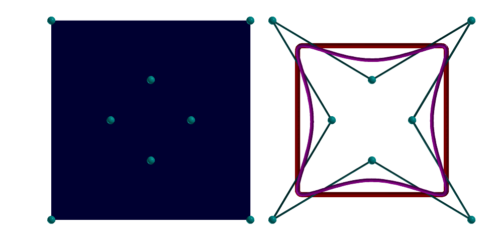
FIGURE: A convex hull of a set of points and of a freeform B-spline curve. The left show a convex hull of a set of points. The right shows the convex hull (thick line) of a freeform curve.
COERCE
AnyType COERCE( AnyType Object, ConstantType NewType )
provides a coercion mechanism between different objects or object types. PointType, VectorType, PlaneType, and CtlPtType can be all coerced to each other by using the NewType of POINT_TYPE, VECTOR_TYPE, PLANE_TYPE, or one of E1-E9, P1-P9 (CtlPtType). Similarly, CurveType, SurfaceType, TrimSrfType, TriSrfType, TrivarType, and MultivarType can all be coerced to hold different CtlPtType control points, or even different open end conditions from KV_PERIODIC to KV_FLOAT to KV_OPEN. Freefroms can be coerced to a Power, Bezier or a B-spline type via the NewType of POWER_TYPE, BEZIER_TYPE or the BSPLINE_TYPE. If a scalar (E1 or P1) curve is coerced to E2 or P2 curve or a scalar (E1 or P1), the surface is coerced to an E3 or P3 surface, and the Y (YZ) coordinate(s) is (are) updated to hold the parametric domain of the curve (surface). That is X = U (Y = V). Curves, Surfaces, and Trivariates can be coerced to/from Multivariates using the CURVE_TYPE, SURFACE_TYPE, TRIVAR_TYPE and MULTIVAR_TYPE. Trimmed B-spline surfaces can ve coerced to trimmed Bezier surfaces via a BEZIER_TYPE coercion and to untrimmed tensor product pieces using UNTRIMMED_TYPE. Models can be coerced to surfaces and trimmed surfaces, and VModels can be coerced to trimmed surfaces, to Models, or to individual volumetric elements that are trimmed trivariates (VElements of VModels), when coerced to themselves (to VModels). Surfaces and trimmed surfaces can be coerced to Models and VModels (if closed) and trivariates (possibly with "Model" attribute of a Boundary model) can be coerced to VModels. The coercion of geometry to its own type has no effect except for SurfaceType where duplicated surfaces are removed. VElements of VModels can be further subdivided into Bezier trimmed trivariates if coerced to BEZIER_TYPE.
Example:
    CrvE2 = COERCE( Crv, E2 );
    MultiVar == COERCE( COERCE( MultiVar, surface_type ), multivar_type );
    BzrSrfs = COERCE( BspSrf, bezier_type );
coerces Crv to a new curve that will have an E2 CtlPtType control points. Coerction of a projective curve (P1-P9) to a Euclidean curve (E1-E9) does not preseve the shape of the curve. The second example coerces a bivariate MultiVar into a Srf and back and compares the result to the original multivariate MultiVar... The third example coerces a B-spline surface BspSrf to a Bezier form, returning one or more Bezier surfaces representing the same geometry as BspSrf.
COFFSET
 AnyType COFFSET( CurveType Crv, Numericype Offset,
                  Numericype Operation, Numericype Eps )
computes an offset approximation of a planar curve Crv, by offset amount Offset, to an accuracy of Eps, that relates to the square distance between Crv and its offset. Eps can be negative, to request a return of the clipped curve segments. Operation can be one of:
| 0 | return valid curve segments in original curve. |
|---|---|
| 1 | return valid curve segments as offset curves |
| 2 | merge the offset curve segments (as in Operation = 1) |
| into one final offset curve. |
Example:
ofstC = coffset( c, 0.1, 2, 0.001 ):
See also OFFSET, AOFFSET, TOFFSET, LOFFSET, and MOFFSET.
COMPOSE
 CurveType COMPOSE( CurveType Crv1, CurveType Crv2 )

 or

 CurveType COMPOSE( SurfaceType Srf, CurveType Crv )
 CurveType COMPOSE( SurfaceType Srf, CurveType Crv, NumerType Periodic )

 or

 SurfaceType COMPOSE( SurfaceType Srf1, SurfaceType Srf2 )

 or

 CurveType COMPOSE( TrivarType TV, SurfaceType Crv )

 or

 SurfaceType COMPOSE( TrivarType TV, SurfaceType Srf )

 or

 SurfaceType COMPOSE( MultivarType MV1, MultivarType MV2 )
 SurfaceType COMPOSE( MultivarType MV1, MultivarType MV2, ListType DimMap )
symbolically compute the composition curve or surface. In the above first form of Crv1(Crv2(t), Crv1 can be any curve while Crv2 is assumed to be a one-dimensional curve that is either E1 or P1 (higher dimensions are ignored). In the above second form of Srf(Crv(t)), the Srf can be any surface, while the Crv is assumed to be a two-dimensional curve, that is either E2 or P2 (higher dimensions are ignored). If a third optional parameter Periodic is specified, it sets if the surface is considered periodic in its domain (if TRUE) or not. If this parameter is not specified periodicity is not assumed. In the above third form of Srf1(srf2(u, v)), Srf2 can be any surface, while it is assumed to be a two-dimensional surface, that is either E2 or P2 (higher dimensions are ignored). Srf1 is a Bezier. In the above fourth form of TV(Crv(t)), the Crv can be any curve, while it is assumed to be a three-dimensional curve, that is either E3 or P3 (higher dimensions are ignored). TV is a Bezier. In the above fifth form of TV(Srf(u, v)), the Srf can be any surface, while it is assumed to be a three-dimensional surface, that is either E3 or P3 (higher dimensions are ignored). TV is a Bezier. In the sixth form of MV1(MV2), two general multivariates are composed. It is allowed for the range of MV2 to be a sub-domain of MV1, in which case DimMap is a list object of dimensions in MV1 to map the range of MV2 into. In other words, the range of MV2 is of size sizoef(DimMap). The second freeform must always be fully contained in the first freeform's parametric domain, up to the periodicity described above.
Example:
   srf = sbezier( list( list( ctlpt( E3, 0.0, 0.0, 0.0 ),
                              ctlpt( E3, 0.0, 0.5, 1.0 ),
                              ctlpt( E3, 0.0, 1.0, 0.0 ) ),
                        list( ctlpt( E3, 0.5, 0.0, 1.0 ),
                              ctlpt( E3, 0.5, 0.5, 0.0 ),
                              ctlpt( E3, 0.5, 1.0, 1.0 ) ),
                        list( ctlpt( E3, 1.0, 0.0, 1.0 ),
                              ctlpt( E3, 1.0, 0.5, 0.0 ),
                              ctlpt( E3, 1.0, 1.0, 1.0 ) ) ) );
   crv = circle( vector( 0.5, 0.5, 0.0 ), 0.4 );
   comp_crv = COMPOSE( srf, crv );
composes a circle Crv to be on the surface Srf. See figure for an example.
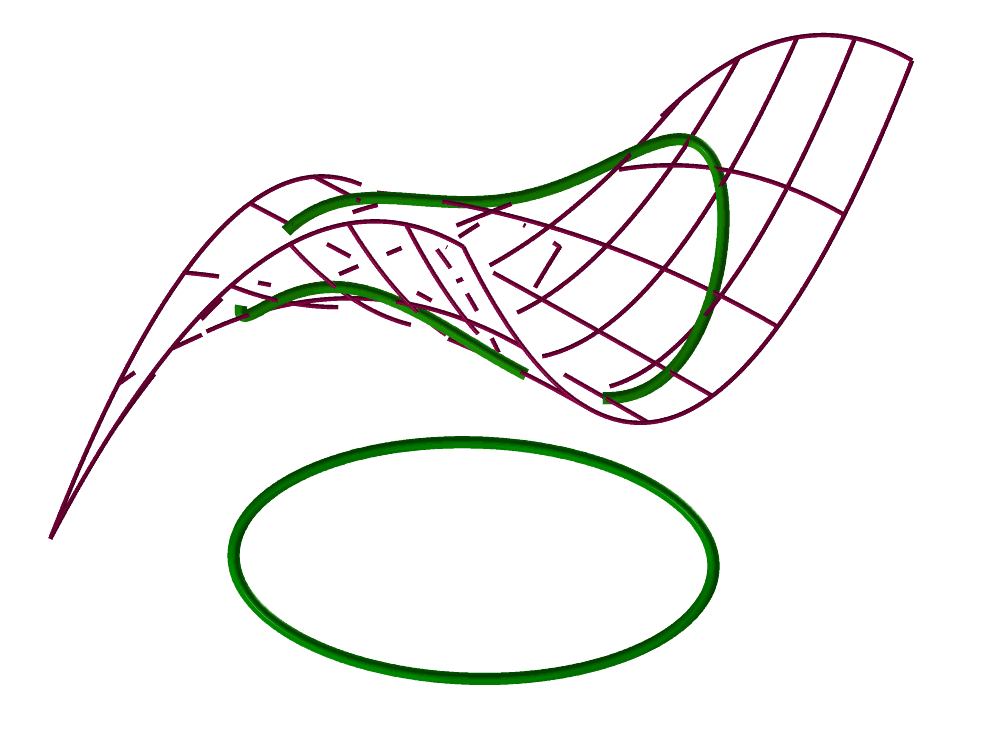
FIGURE: A circle in the parametric space of the freefrom surface is composed to create a closed loop curve on the surface using COMPOSE.
See also TDEFORM.
CON2
 PolygonType CON2( VectorType Center, VectorType Direction,
                   NumericType Radius1, NumericType Radius2,
                   NumericType Caps )
creates a truncated CONE geometric object, defined by Center as the center of the main base of the CONE, with the Direction as both the CONE's axis and the length of CONE, and the two radii Radius1/2 of the two bases of the CONE. If Caps equals zero, no caps are created. If Caps equal one (two), only the bottom (top) cap is created. If Caps equal three, both the top and the bottom caps are created.
Unlike the regular cone (CONE) constructor which inherits discontinuities in its generated normals at the apex, CON2 can be used to form a (truncated) cone with continuous normals. See RESOLUTION for the accuracy of the CON2 approximation as a polygonal model. See also CONE. See IRITSTATE's "PrimRatSrfs" and "PrimRatSrfs" state variables.
Example:
Cone2 = CON2( vector( 0, 0, -1 ), vector( 0, 0, 4 ), 2, 1, 3 );
constructs a truncated cone with bases parallel to the XY plane at Z = -1 and Z = 3, and with radii of 2 and 1 respectively. Both caps are created. See figure for an example.
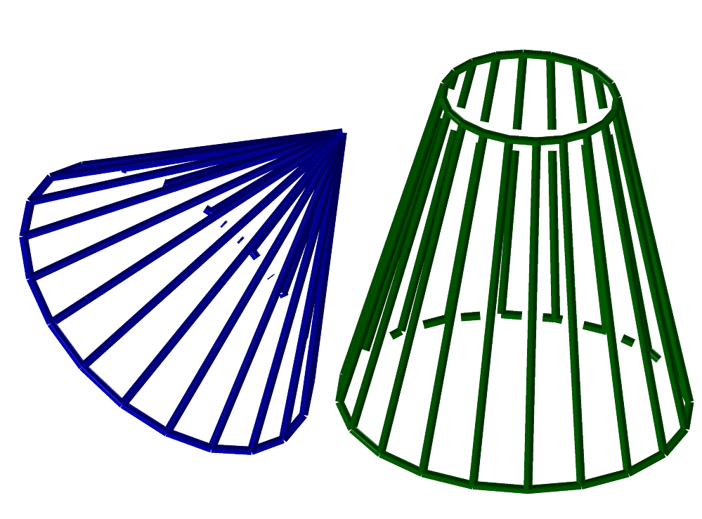
FIGURE: A cone (left) can be constructed using the CONE constructor and a truncated cone (right) using the constructor CONE2.
CONE
 PolygonType CONE( VectorType Center, VectorType Direction,
                   NumericType Radius, NumericType Caps )
creates a CONE geometric object, defined by Center as the center of the base of the CONE, Direction as the CONE's axis and height, and Radius as the radius of the base of the CONE. If Caps equals zero, no cap is created. If Caps equal one, the bottom (top) cap is created. See RESOLUTION for accuracy of the CONE approximation as a polygonal model.
Example:
Cone1 = CONE( vector( 0, 0, 0 ), vector( 1, 1, 1 ), 1, 1 );
constructs a cone based in an XY parallel plane, centered at the origin with radius 1 and with tilted apex at ( 1, 1, 1 ). Only the bottom cap is created.
See IRITSTATE's "PrimRatSrfs" and "PrimRatSrfs" state variables. See also CON2. See figure for an example.
CONICSEC
 CurveType CONICSEC( ListType ABCDEF,
                     NumericType ZLevel,
                     PointType StartPoint,
                     PointType EndPoint )

 or

 {PolygonType | SurfaceType } CONICSEC( ListType TwoCurves,
                                        NumericType ZLevel,
                                        NumericType Dist,
                                        NumericType EvalCurve )
In the first form, this will construct a quadratic form that represents the planar conic section prescribed by the list of six coefficients ABCDEF as:
A x^2 + B xy + C y^2 + D x + E y + F = 0,The conic will be parallel to the XY plane at Z level of Zlevel. The section of the curve will be from StartPoint to EndPoint, or alternatively, unlimited by specifying 'off' for StartPoint and EndPoint. The conic might be rational (for circles and ellipses, for example) or intergral (for parabolas).
Alternatively, in the second form, if the first list object parameter contains two planar curves in the XY plane, a piecewise linear curve at Z level of Zlevel is computed that presents the elliptic/hyperbolic distance Dist from the given two curves. The elliptic distance refers to the sum of distance (that equal Dist) to the two curves, while hyperbolic distance refers to the difference of distances. Finally, if EvalCurve = 0, the surface whose zero set is the desired curve, is returned instead. If EvalCurve = 1, distance curves are returned in the parametric space as correspondence between the two curves' parameters. If EvalCurve = 2, the conic curves themselves are returned. Note only elliptic surfaces are compact and are reconstructed in whole.
Example:
    Circ2 = CONICSEC( list( 1, 0, 1, 0, -0.5, -1 ), 0.0,
                      point(  1.0, 0.0, 0.0 ) * ty( 0.25 ),
                      point( -0.707, -0.707, 0.0 ) * ty( 0.25 ) );
    Elp1 = CONICSEC( list( 1, 2, 4, 0.5, 2, -0.2 ), 0.0, off, off );
    Prb1 = CONICSEC( list( 0.1, 0, 0, 0, 1, -1 ), 2, off, off ) * sc( 0.1 );
constructs a (portion of a) circle, an ellipse and a parabola as conic sections, and,
    c1 = cbspline( 3,
                   list( ctlpt( E2, -1, -1 ),
                         ctlpt( E2,  1, -1 ),
                         ctlpt( E2,  1,  1 ),
                         ctlpt( E2, -1,  1 ) ),
                   list( KV_OPEN ) );
    c2 = -c1 * sx( -1 ) * tx( 5 );
    view( list( c1, c2 ), 1 );

    resolution = 15;

    DistCrvE = list( CONICSEC( list( c1, c2 ), 1.0, 10, 2 ),
                     CONICSEC( list( c1, c2 ), 1.0,  9, 2 ),
                     CONICSEC( list( c1, c2 ), 1.0,  8, 2 ),
                     CONICSEC( list( c1, c2 ), 1.0,  7, 2 ),
                     CONICSEC( list( c1, c2 ), 1.0,  6, 2 ) );
    color( DistCrvE, green );
computes the conic distance to the two curves c1 and c2 at distances of 6, 7, 8, 9, and 10.
See also QUADRIC.
CONTOUR
 PolygonType CONTOUR( SurfaceType ContouredSrf, PlaneType ContourPlane,
                      NumericType SubdivTol )

 or

 PolygonType CONTOUR( SurfaceType ContouredSrf, PlaneType ContourPlane,
                      NumericType SubdivTol, SurfaceType MappedSrf )

 or

 PolygonType CONTOUR( SurfaceType ContouredSrf, PlaneType ContourPlane,
                      NumericType SubdivTol, SurfaceType MappedSrf,
                      ListType ValidatePt )
contours surface ContouredSrf by intersecting plane ContourPlane with ContouredSrf. If SubdivTol < 1, the contours are derived using the multivariate solver and SubdivTol controls the subdivision accuracy. If SubdivTol > 1 a polygonal approximating of ContouredSrf} is first derived and then polygon-polygon intersections are computed. If ContouredSrf is a scalar field surface of type E1 or P1 and MappedSrf is provided, ContouredSrf is contoured above its parametric domain (U is X, V is Y) and the resulting parametric curve is composed with MappedSrf to yield the returned value. Further, if ValidatePt is prescribed, it should contain two elements, a vector, V, and an angle, A, in degrees. Only the contour points for which the normal of surface MappedSrf there has less than A degrees from V are returned.
Example:
 resolution = 20;
 nglass = snrmlsrf( glass ) * vector( 1, 1, 1 );

 sils = contour( nglass, plane( 1, 0, 0, 0 ), 1e-3, glass );
 color( sils, cyan );
 attrib( sils, "dwidth", 4 );

 view( list( axes, glass, sils ), on );
computes the normal field of the surface glass, projects it onto the viewing direction of (1, 1, 1) and contours the resulting scalar field with the plane X = 0, to extract the silhouette curves from viewing direction (1, 1, 1). See figure for an example.
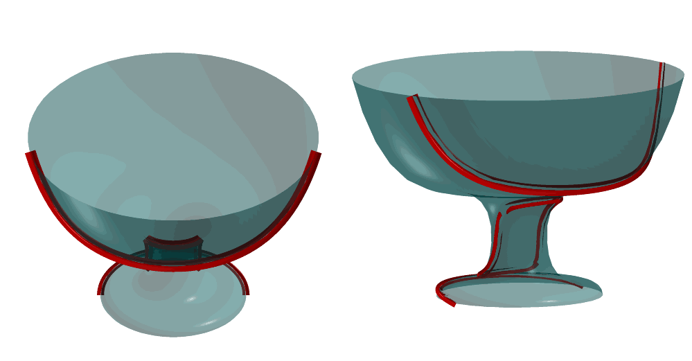
FIGURE: Computes the silhouette of a freeform glass surface from viewing direction (1, 1, 1). On the left, the original view is seen. On the right, a different, general, view is provided.
CONVEX
 PolygonType CONVEX( PolygonType Object )

 or

 ListType CONVEX( ListType Object )
convert non-convex polygons in Object, into convex ones. New vertices are introduced into the polygonal data during this process. The Boolean operations require the input to have convex polygons only (although it may return non convex polygons...) and it automatically converts non-convex input polygons into convex ones, using this same routine.
However, some external tools (such as irit2ray and poly3d-h) require convex polygons. This function must be used on the objects to guarantee that only convex polygons are saved into data files for these external tools.
Example:
    CnvxObj = CONVEX( Obj );
    save( "data", CnvxObj );
converts non-convex polygons into convex ones, so that the data file can be used by external tools requiring convex polygons.
COORD
AnyType COORD( AnyType Object, NumericType Index )
extracts an element from a given Object, at index Index. From a PointType, VectorType, PlaneType, CtlPtType and MatrixType. A NumericType is returned with Index 0 for the X axis, 1 for the Y axis etc. Index 0 denotes the weight of CtlPtType. For a PolygonType that contains more than one polygon, the Indexth polygon is returned. For a PolygonType that contains a single Polygon, the Indexth vertex is returned. For a freeform object (curve, surface, etc.), the Indexth CtlPtType is returned. For a ListType, COORD behaves like NTH and returns the Indexth object in the list. For a StringType, the Indexth character is returned as its ASCII numeric code.
Example:
    a = vector( 1, 2, 3 );
    vector( COORD( a, 0 ), COORD( a, 1 ), COORD( a, 2 ) );

    a = ctlpt( P2, 6, 7, 8, 9 );
    ctlpt( P3, coord( a, 0 ), coord( a, 1 ), coord( a, 2 ), coord( a, 3 ) );

    a = plane( 10, 11, 12, 13 );
    plane( COORD( a, 0 ), COORD( a, 1 ), COORD( a, 2 ), COORD( a, 3 ) );
constructs a vector/ctlpt/plane and reconstructs it by extracting the constructed scalar components of the objects using COORD.
See also COERCE.
COVERISO
 CurveType COVERISO( TrivarType TV,
                     NumericType NewOfStrokes,
                     NumericType StrokeType,
                     PointType MinMaxPwrLen,
                     NumericType StepSize,
                     NumericType IsoVal,
                     VectorType ViewDir )
computes a coverage for an iso surface of a trivariate function TV, using curves. NewOfStrokes strokes are distributed on the iso surface with a length that is set via MinMaxPwrLen. MinMaxPwrLen is a triplet of the form (Min, Max, Power) that determines the length of the strokes as,
Avg = (Max + Min) / 2, Dev = (Max - Min) / 2
Length = Avg + Dev * Random(0, 1) ^ Pwr.StepSize controls the steps size of the piecewise linear approximation formed and should typically be smaller than Min. StrokeType can be one of,
| 1 | Draw strokes along minimal principal curvature. |
|---|---|
| 2 | Draw strokes along maximal principal curvature. |
| 3 | Draw strokes along both principal curvatures. |
| 4 | Draw strokes along constant X planes. |
| 5 | Draw strokes along constant Y planes. |
| 6 | Draw strokes along constant Z planes. |
Example:
    IsoVal = 0.12;
    Cover = CoverIso( ThreeCyls, 500, 1, vector( 3, 10, 1.0 ), 0.2, IsoVal );
draws 500 strokes on the iso surface of trivariate ThreeCyls at iso value IsoVal and step size of 0.2. Strokes are drawn in length of 3 to 10 along lines of curvatures of minimal curvature. See figure for an example.
FIGURE: A uniform coverage of 500 curved strokes of an iso surface of a trivariate function, computed using COVERISO command.
COVERPT
 PolygonType COVERPT( PolygonType Model,
                      NumericType NumOfPts,
                      VectorType ViewDir )
computes a uniform point distribution on the given polygonal Model. Approximately NumOfPts points are uniformly distributed on the model's surface, provided ViewDir is the zero vector. If ViewDir is a non zero vector, the distribution is made to be uniform from this given viewing direction. In all cases, NumOfPts is an upper bound of the the real number of distributed points, which will be in the same order.
See also SADAPISO, COVERISO, FFPTDIST.
Example:
    Pts1 = CoverPt( solid1, 1000, vector( 0, 0, 0 ) );
    Pts2 = CoverPt( solid1, 3000, vector( 0, 0, -1 ) );
computes two uniform distributions of 1000 and 3000 points on Solid1. Pts1 is uniform in three space, while Pts2 is viewed uniform from the -Z direction.
See figure for an example.
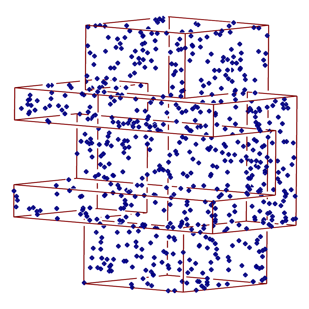
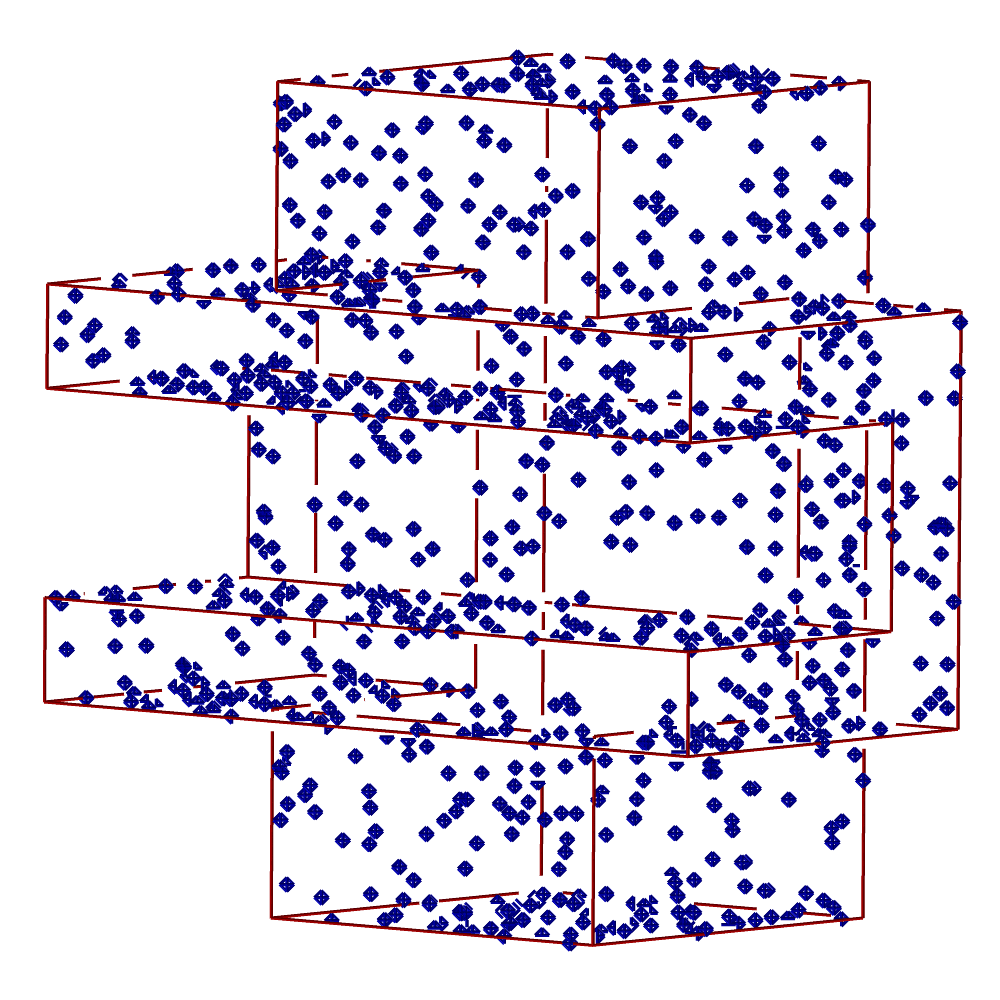
FIGURE: A uniform coverage of 1000 and 3000 points of a polygonal model in three space, computed using the COVERPT command. On the left, the distribution is directional, from the viewing direction, while on the right, shows a point distribution that is uniform in 3-space. Distant points are smaller, emulating point depth cueing.
CPINCLUDE
NumericType CPINCLUDE( CurveType Crv, PointType Pt, NumericType Tol )
tests if a point Pt is inside a 2D closed curve Crv. Returns +1 if inside, -1 if outside, and 0 if on the boundary to within Tol. Tol governs the tolerance of the computations.
Example:
    if ( CPINCLUDE( Crv, pt ) > 0,
         ... );
See also PPINCLUDE.
CPOWER
CurveType CPOWER( ListType CtlPtList )
creates a polynomial/rational curve out of the provided control point list. The created curve is employing the monomial power basis. CtlPtList is a list of control points, all of which must be of type (E1-E9 P1-P9), or regular PointType defining the curve's control polygon. The curve's point type will be of a space which is the union of the spaces of all points.
Example:
 c = CPOWER( list( ctlpt( E3, 0, 1, 0 ),
                   ctlpt( E3, 1, 0, 0 ),
                   ctlpt( E3, 0, 0, 1 ) ) );
 c == coerce( coerce( c, bezier_type ), power_type );
constructs a quadratic power basis curve, coerces it to a Bezier form, coerces the Bezier form back to the power basis, and then compares the result for equality.
See also CBEZIER, CBSPLINE and SPOWER.
CRAISE
CurveType CRAISE( CurveType Curve, NumericType NewOrder )
Raise Curve to the NewOrder Order specified.
Example:
    Crv = cbezier( list( ctlpt( E2, -0.7,  0.3 ),
                         ctlpt( E2,  0.0,  1.0 ),
                         ctlpt( E2,  0.7,  0.0 ) ) );
    Crv2 = CRAISE( Crv, 5 );
raises the 90 degrees corner Bezier curve Crv to be a quadratic. See figure for an example.
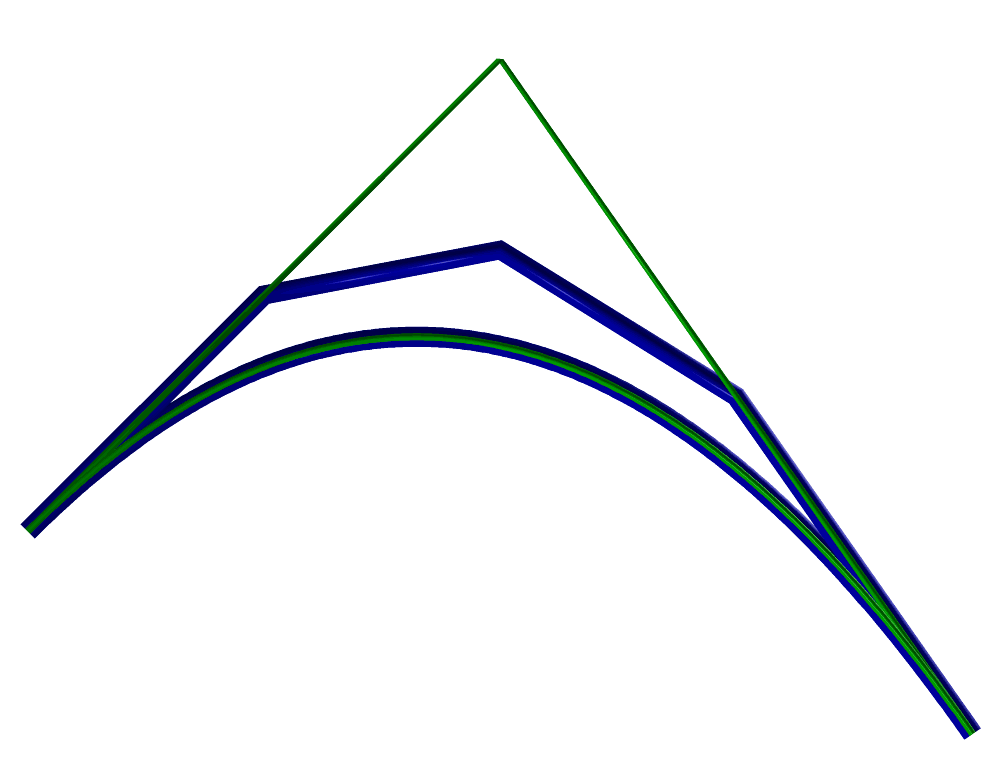
FIGURE: Raises a 90 degrees corner quadratic Bezier curve to a quintic using CRAISE. The control polygons are also shown.
See also CREDUCE, TRAISE, SRAISE, and MRAISE.
CRC2CRVTAN
 ListType CRC2CRVTAN( CurveType Crv1, CurveType Crv2,
                      NumericType Radius, NumericType Tol )
computes all circles that are bi-tangent to the given two curves Crv1 and Crv2. The circles will posses a radius of Radius. The accuracy of the computation is governed by the tolerance Tol. Returned is a list center point locations with "Params" attributes of parameter values of the tangent locations at the two curves.
Example:
Cntrs = CRC2CRVTAN( c1, c2, R, 1e-3 );
computes all the circles of radius 0.1 that are bi-tangent to the two curves c1 and c2. Tolerance of computation is 1e-3. See figure for an example.
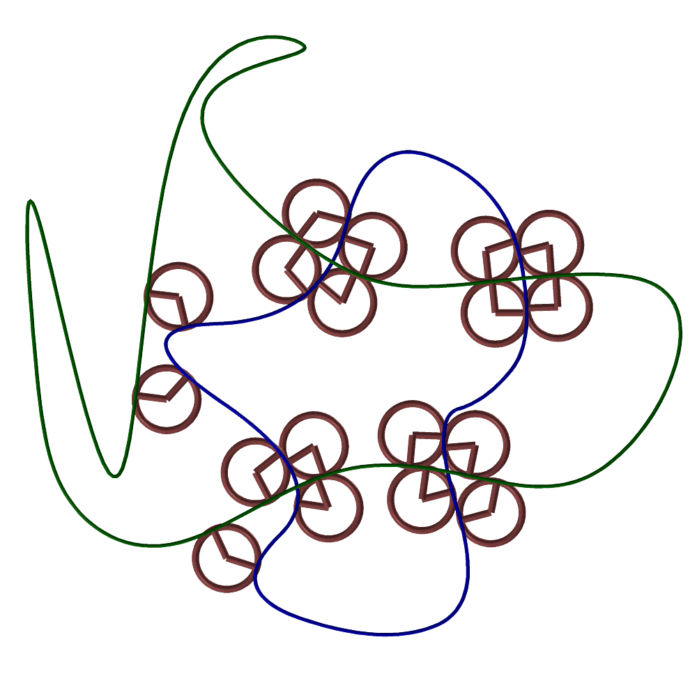
FIGURE: Computes all the bi-tangent circles to the given two curves via the CRC2CRVTAN function.
See also SKEL2DINT, CRV2TANS, TNSCRCR, CRVC1RND.
CREDUCE
CurveType CREDUCE( CurveType Curve, NumericType NewOrder )
reduces the Curve to the NewOrder Order specified. This function approximates the lower order curve in the infinity norm sense, minimizing the maximal deviation between the original curve Curve and the low order curve NewOrder. NewOrder will identify with Curve only if Curve was degree raised before.
Example:
    Crv = cbezier( list( ctlpt( E2, -0.7,  0.3 ),
                         ctlpt( E2,  0.0,  1.0 ),
                         ctlpt( E2,  0.7,  0.0 ) ) );
    Crv2 = CREDUCE( craise( Crv, 5 ), 3 );
    Crv == Crv2;
Should restore the original quadratic order. I.e. Crv2 should identify with Crv and "Crv == Crv2;" should return TRUE.
See also CRAISE.
CREFINE
CurveType CREFINE( CurveType Curve, NumericType Replace, ListType KnotList )
provides the ability to Replace a knot vector of Curve, or refine it. KnotList is a list of knots at which to refine Curve. All knots should be contained in the parametric domain of the Curve. If the knot vector is replaced, the length of KnotList should be identical to the length of the original knot vector of the Curve. If Curve is a Bezier curve, it is automatically promoted to be a B-spline curve.
Example:
Crv2 = CREFINE( Crv, FALSE, list( 0.25, 0.5, 0.75 ) );
refines Crv and adds three new knots at 0.25, 0.5, and 0.75. See figure for an example.
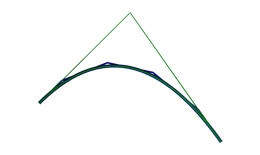
FIGURE: Refines a 90 degrees corner quadratic Bezier curve at three interior knots (the result is a B-spline curve) using CREFINE. The control polygons are also shown.
See also SREFINE, TREFINE, and MREFINE.
CREGION
 CurveType CREGION( CurveType Curve, NumericType MinParam,
                                                       NumericType MaxParam )
extracts a region from the Curve between MinParam and MaxParam. Both MinParam and MaxParam should be contained in the parametric domain of the Curve, except for Bezier curves when MinParam and MaxParam can be arbitrary (extrapolating if not between zero and one).
Example:
SubCrv = CREGION( Crv, 0.3, 0.6 );
extracts the region from the Crv from the parameter value 0.3 to the parameter value 0.6. See figure for an example.
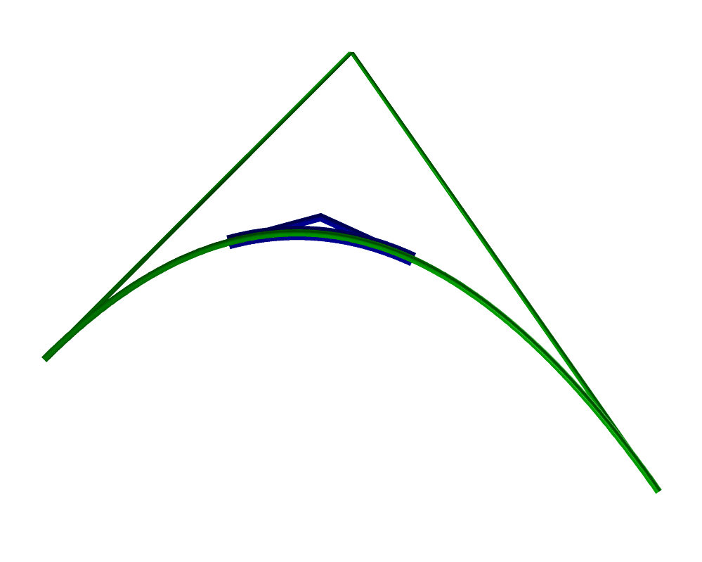
FIGURE: Extracts a sub region from a curve using CREGION.
See also SREGION, TREGION, and MREGION.
CREPARAM
 CurveType CREPARAM( CurveType Curve, NumericType MinParam,
                                                       NumericType MaxParam )
reparametrizes the Curve over a new domain from MinParam to MaxParam. This operation does not affect the geometry of the curve and only affine transforms its knot vector. A Bezier curve will automatically be promoted into a B-spline curve by this function.
If MinParam equals MaxParam and both equates with one of the parameterization keywords of PARAM_UNIFORM, PARAM_CENTRIP, PARAM_CHORD, or PARAM_NIELFOL, then that parametrization is approximated for the curve, by changing the knot sequence. Note this last operation affects the geometry of the curve.
Example:
    arc1 = arc( vector( 0.0, 0.0, 0.0 ),
                vector( 0.5, 2.0, 0.0 ),
                vector( 1.0, 0.0, 0.0 ) );
    crv1 = arc( vector( 1.0, 0.0, 0.75 ),
                vector( 0.75, 0.0, 0.7 ),
                vector( 0.5,  0.0, 0.85 ) ) +
           arc( vector( 0.5,  0.0, 0.75 ),
                vector( 0.75, 0.0, 0.8 ),
                vector( 1.0,  0.0, 0.65 ) );

    arc1 = CREPARAM( arc1, 0, 10 );
    crv1 = CREPARAM( crv1, 0, 10 );
sets the domain of the given two curves to be from zero to ten. The Bezier curve arc1 is promoted to a B-spline curve. See also SREPARAM, TREPARAM, and MREPARAM.
CROSSEC
PolygonType CROSSEC( PolygonType Object )
This feature is NOT implemented.
CRV2TANS
 ListType CRV2TANS( CurveType Crv, NumericType FineNess )

 or

 ListType CRV2TANS( ListType TwoCrvs, NumericType FineNess )
computes all the self bi-tangents of a Crv or all bi-tangents between TwoCrvs, in the XY plane. That is, all lines that are tangent to Crv at two different locations. A list of points with X and Y coefficients representing the two parametric locations on Crv or on TwoCrvs of the bi-tangent is returned. FineNess controls the numerical accuracy (sploution separation) of the computation. A value of 0.01 will provide a good start and the smaller this number is, the better the accuracy will be. See also CRVPTTAN and CNVXHULL.
Example:
    Tans = nil();
    Crv2Tns = Crv2Tans( Crv, 0.01 );
    for ( i = 1, 1, sizeof( Crv2Tns ),
        pt = nth( Crv2Tns, i ):
        snoc( ceval( Crv, coord( pt, 0 ) ) +
              ceval( Crv, coord( pt, 1 ) ), Tans ) );
finds the bi-tangents of Crv and converts them to a set of line segments. See figure for an example.
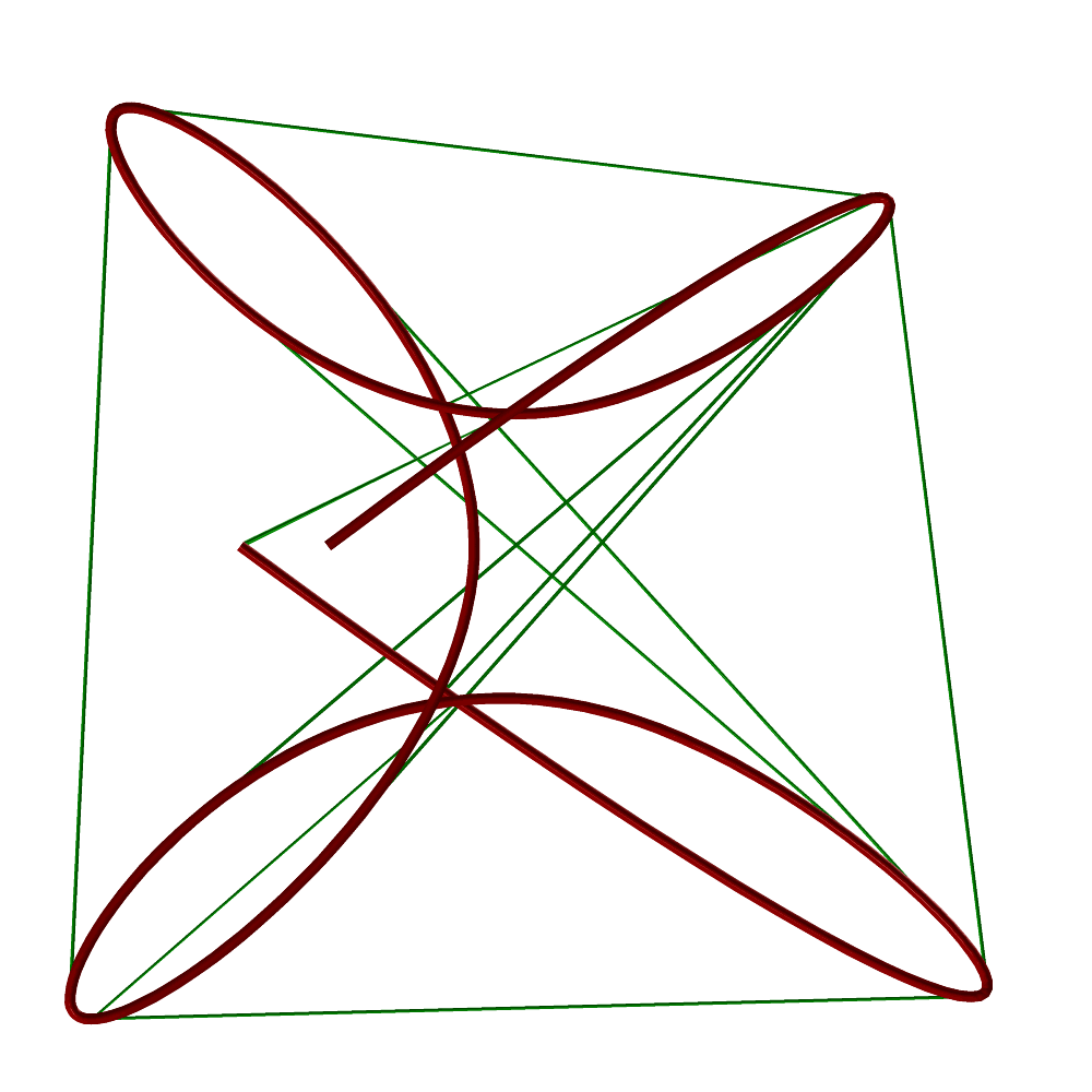
FIGURE: Computes the bi-tangents of a freeform curve, using CRV2TANS.
See also CRC2CRVTAN, TNSCRCR, SKEL2DINT.
CRVBUILD
CurveType CRVBUILD( NumerticType BuildOp, ListType Params )
Constructs a planar B-spline curve incrementally, specifying one (control) point at a time. BuildOp specifies the next incremental curve build operation whereas Params prescribes the parameters of that specific BuildOp.
In the following, all angles are in degrees. Some operations add new points relative to previous ones - if no previous location is set yet, (0, 0) is asssumed.
The different BuildOp operations are:
| 0 | INIT - Initialized the incremental construction. |
|---|---|
| No parameters are expected. | |
| 1 | XY - Appends a new XY location. Expects (X, Y) as Params. |
| 2 | X - Appends a new XY location. Expects (X) as Params (Y |
| is same as last point). | |
| 3 | Y - Appends a new XY location. Expects (Y) as Params (X |
| is same as last point). | |
| 4 | DELTA_XY - Appends a new XY location. Expects |
| (DeltaX, DeltaY) as Params, as relative locations to | |
| previous location. | |
| 5 | DELTA_X - Appends a new XY location. Expects (DeltaX) as |
| Params, as relative location to previous X location. | |
| Y is same as last point. | |
| 6 | DELTA_Y - Appends a new XY location. Expects (DeltaY) as |
| Params, as relative location to previous Y location. | |
| X is same as last point. | |
| 7 | DELTA_X_AND_Y - Appends a new XY location. Expects |
| (DeltaX, Y) as Params. A new Y location and a relative | |
| X location to previous X. | |
| 8 | DELTA_Y_AND_X - Appends a new XY location. Expects |
| (X, DeltaY) as Params. A new X location and a relative | |
| Y location to previous Y. | |
| 9 | DIST_ALPHA - Appends a new XY location. Expects |
| (d, Alpha) as Params. A new XY location relative to last | |
| location in polar coordinates as (d cos(Alpha), d sin(Alpha)). | |
| 10 | DIST_DELTA_ALPHA - Appends a new XY location. Expects |
| (d, DeltaAlpha) as Params. A new XY location relative to | |
| last location in polar coordinates as | |
| (d cos(LastAlpha + DeltaAlpha), d sin(LastAlpha + DeltaAlpha). | |
| 11 | DELTA_X_DELTA_ALPHA - Appends a new XY location. Expects |
| (DeltaX, DeltaAlpha) as Params. Seeks a new XY location | |
| in direction LastAlpha + DeltaAlpha until it intersects | |
| the line X = LastX + DeltaX. | |
| 12 | DELTA_Y_DELTA_ALPHA - Appends a new XY location. Expects |
| (DeltaY, DeltaAlpha) as Params. Seeks a new XY location | |
| in direction LastAlpha + DeltaAlpha until it intersects | |
| the line Y = LastY + DeltaY. | |
| 13 | ALPHA_LINE - Appends a new XY location. Expects |
| (Alpha, X2, Y2, Alpha2) as Params. Seeks a new XY location | |
| in direction Alpha from current location at the intersection | |
| with the linedefined by (X, Y) in direction Alpha2. | |
| 14 | ARC - Modifies the last XY location. Expects (R, F) as Params. |
| Replaces the last segment with an arc that ends at the two | |
| end points of the segment. Positive R(ad) for an arc on the | |
| left, Negative on the right. If F(lipped) is non zero, the | |
| other left/right arc is provided (note there are four ways | |
| to connect two points with C/CW arcs). | |
| 15 | ADD_INTERMEDIATE - Modifies last XY location. Expects |
| (A, D, W) as Params. Adds interior (control) points to the | |
| last segment. A is between zero and one setting the | |
| distance along the segment (A = 0 starting point, | |
| 1 end point). D is the signed distance (positive for the | |
| left size) orthogonal to the line segment. Finally W sets | |
| the weight of the new (control) points. | |
| This feature enable the creation of arbitrary degree spline | |
| curves. if all W are 1.0, a polynomial curve is created. | |
| 16 | ROUND_LAST - Rounds the last entered point. Expects (R) |
| as the parameter, the radius of the round. | |
| 17 | CHAMFER_LAST - Chamfers the last entered point. Expects (C) |
| as the parameter, the size of the chamfer, that linearly | |
| connects the two tangency points of a rounding of size C. | |
| 18 | CURVE_PARAMS - Sets default curve parameters. Expects |
| (d, KV) as Params. The parameter d sets the degree of | |
| the constructed curve (if the construction requires a | |
| higher degree a higher degree will be used). KV sets the | |
| knot sequence to use which is one of uniform open (0), | |
| uniform float (1), or uniform periodic (2). | |
| 19 | CLOSE - Terminate the constriction. Expects (P, d) as |
| Params. If P is negative the shape is closed to the initial | |
| location. If P is positive an open curve will be created. | |
| If P = +/-2 all sharp corners are going to be chamfered as | |
| controlled by d. If P = +/-3 all sharp corners | |
| will be rounded by radius d. |
 CAGD_CRV_INC_CNSTRCT_INIT = 0:
 CAGD_CRV_INC_CNSTRCT_XY = 1:
 CAGD_CRV_INC_CNSTRCT_X = 2:
 CAGD_CRV_INC_CNSTRCT_Y = 3:
 CAGD_CRV_INC_CNSTRCT_DELTA_XY = 4:
 CAGD_CRV_INC_CNSTRCT_DELTA_X = 5:
 CAGD_CRV_INC_CNSTRCT_DELTA_Y = 6:
 CAGD_CRV_INC_CNSTRCT_DELTA_X_AND_Y = 7:
 CAGD_CRV_INC_CNSTRCT_DELTA_Y_AND_X = 8:
 CAGD_CRV_INC_CNSTRCT_DIST_ALPHA =  9:
 CAGD_CRV_INC_CNSTRCT_DIST_DELTA_ALPHA = 10:
 CAGD_CRV_INC_CNSTRCT_DELTA_X_DELTA_ALPHA = 11:
 CAGD_CRV_INC_CNSTRCT_DELTA_Y_DELTA_ALPHA = 12:
 CAGD_CRV_INC_CNSTRCT_ALPHA_LINE = 13:
 CAGD_CRV_INC_CNSTRCT_ARC = 14:
 CAGD_CRV_INC_CNSTRCT_ADD_INTERMEDIATE = 15:
 CAGD_CRV_INC_CNSTRCT_ROUND_LAST = 16:
 CAGD_CRV_INC_CNSTRCT_CHAMFER_LAST = 17:
 CAGD_CRV_INC_CNSTRCT_CURVE_PARAMS = 18:
 CAGD_CRV_INC_CNSTRCT_CLOSE = 19:
 CAGD_CRV_INC_CNSTRCT_DEBUG = 20;

 CrvBuild( CAGD_CRV_INC_CNSTRCT_INIT, nil() );
 CrvBuild( CAGD_CRV_INC_CNSTRCT_XY, list( 0, 0 ) );
 CrvBuild( CAGD_CRV_INC_CNSTRCT_ROUND_LAST, list( 0.1 ) );
 CrvBuild( CAGD_CRV_INC_CNSTRCT_Y, list( 1 ) );
 CrvBuild( CAGD_CRV_INC_CNSTRCT_X, list( 2 ) );
 CrvBuild( CAGD_CRV_INC_CNSTRCT_CHAMFER_LAST, list( 0.45 ) );
 CrvBuild( CAGD_CRV_INC_CNSTRCT_Y, list( 0 ) );

 Crv2 = CrvBuild( CAGD_CRV_INC_CNSTRCT_CLOSE, list( -3, 0.2 ) );
Builds a closed round rectangle spanning (0, 0) to (2, 1), rounded with radius 0.1 at the original, chamfered at (2, 1), and then globally rounded to radius 0.2.
CRVC1RND
CurveType CRVC1RND( CurveType Crv, NumerticType CornerType, NumericTyle Radius )
Give a planar curve Crv with C^1 discontinuities, round (if CornerType is 2) or chamfer (if CornerType is 3) the C^1 discontinuities. Radius controls the rounding (champering) size. If size is too large to fit, no rounding will take place.
Example:
RndCrv = CRVC1RND( Crv, 2, 0.05 );
See figure for an example.
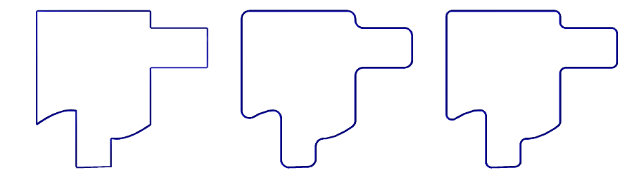
FIGURE: Computes the roundings (middle) and chamfers (right) of the C^1 discontinuous curve on the left, using CRVC1RND.
See also SKEL2DINT, CRV2TANS, TNSCRCR, CRC2CRVTAN.
CRVCOVER
 CurveType CRVCOVER( CurveType DomainBoundary,
                     CurveType InitialCurve,
                     NumericType CoveringTolerance,
                     NumericType NumerTol,
                     NumericType SubdivTol,
                     NumericType NumNewPointsPerIter,
                     NumericType NewPointDistThreshold,
                     NumericType RefinementStrategy )
Covers the given two dimensional domain specified by DomainBoundary} by a random-looking covering curve, upto CoveringTolerance}, so that all points in the domain are at a distance, at most, CoveringTolerance from the computed covering curve. The numeric tolernace and subdivision tolerances are specified by NumerTol and SubdivTol respectively. The maximum number of new points to use in order to refine the covering curve in each iteration is specified by NumNewPointsPerIter. Alternately, one may specify a distance threshold so that only points farther than NewPointDistThreshold from the covering curve are used in refining the curve. The parameterNewPointDistThreshold is used only if NumNewPointsPerIter is negative. The parameter RefinementStrategy} specifies whether to use interpolation or approximation or a blend of the two while refining the covering curve. A value of 1 implies interpolation while 0 implies approximation. Any value in between leads to a blend of the two methods.
Example:
CrvCvr = CRVCOVER( C, 0, 1.50 1e-9, 2e-2, 15, 0.45, 0.5 );
See figure for an example.
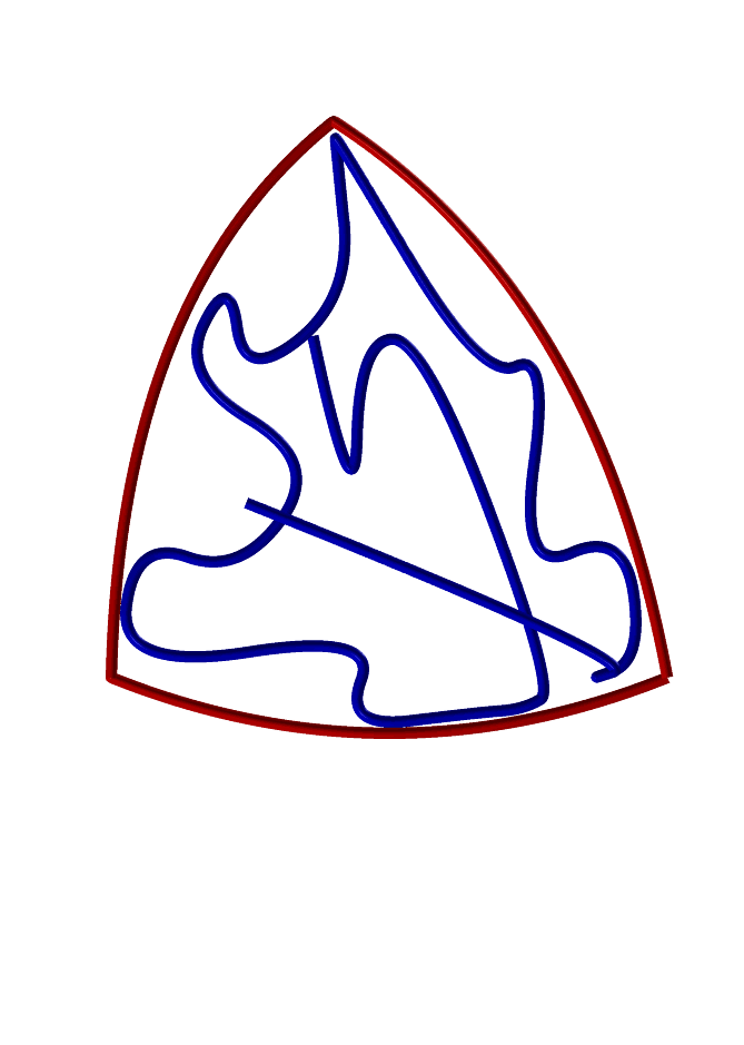
FIGURE: Random covering of a freeform 2D domain with a curve, using CRVCOVER. Boundary is shown in red and the covering curve is shown in blue.
CRVKERNEL
 PolyType | TrivarType | ListType
         CRVKERNEL( CurveType Crv | ListType CrvList,
                    NumericType Gamma, NumericType Euclid,
                    NumericType | ListType KrnlParam, NumericType Mode )
Computes the (gamma) kernel of a given planar curve Crv, or a list of curves CrvList when Mode == 3. If Gamma is zero, the regular kernel is computed. Else, the gamma kernel of Gamma degrees is being computed. If Euclid is TRUE, then the result is returned in the Euclidean space, or if zero, in the parametric space (not used in Mode == 3). Mode can be 0 for a (gamma) kernel solution, 1 to extract silhouette sampling only out of the trivariate function, and 2 for the gamma kernel surface/trivariate functions themselves to be returned. If Mode is 3, a list of kernel points or a convex hull of these points are computed using the inequality constraints, if any.
KrnlParam is a list of control parameters that is specified differently in each mode. When Mode == 0, KrnlParam is either a single numeric value or a list of three numeric values that set the number of knots to insert into the (x,y,t) trivariate functions, t being Crv parameterization, and x, y paramterizes the XY plane as a bbox around Crv. When Mode == 1, KrnlParam is specified as list(SubdivTol, NumericTol), which prescribes the subdivision and numeric tolerances, of the kernel point/silhouette extraction process (See MZERO for their meaning), respectively. When Mode == 2, KrnlParam is the number value that controls the extent of the surfaces/trivariates. When Mode == 3, KrnlParam is specified as list(SubdivTol, OnePt, PreciseBBox, NumTanSamples, CnvxHull), where SubdivTol prescribes the subdivision tolerance, OnePt determines whether to compute only a single kernel point of maximum domain size, or all kernel points, PreciseBBox determines whether to use precise bounding box (when PreciseBBox > 0, the numeric value of PreciseBBox is used as the tolerance of the bounding box computation), NumTanSamples controls the sampling ratio of the tangent lines, which help purging non-kernel domains during subdivision, and CnvxHull determines the form of output. The function returns a list of kernel points if CnvxHull is FALSE, and the convex hull of the kernel points, which is also included in the kernel of the curve(s), otherwise.
Examples:
Krnl = CrvKernel( Crv, 0, 0, list( 2, 3, 1 ), 0 );
computes the regular kernel of curve Crv with a refinement of (2, 3, 1) in the three (x, y, t) axes of the computed trivariate constraint function.
Krnl = CrvKernel( Crv, 0, 1, list( 0.01, 0, 0, 20, TRUE ), 3 );
computes the convex hull of the regular kernel points by subdividing the normalized domain in the bounding box of Crv with the subdivision tolerance of 0.01. To purge non-kernel domains during the subdivision, 20 tangent lines are sampled along Crv.
See also SRFKERNEL.
CRVNET2TILE
 AnyType CRVNET2TILE( ListType CrvList, NumericType DfltOffset,
                      NumericType Tol, NumericType ExtrudeAmount,
                      NumericType OutType )
Constructs a tile to be used in (2D) lattices/microstructures from a list of curves CrvList that intersect. The curves are offseted DfltOffset in both directions (left and right) and all offset curves are intersected, only to build a tiles from this arrangment of curves. Curves in CrvList can have offset curves under them, as attribute "OfstFld", to override the default offsets amount and hence also allow variable distance offset. Tol controls the tolerance of the computation. ExtrudeAmount sets the Z extrusion amount if OutType is trivariate tiles (see below). OutType can be one of 0 to return curves in the plane, 1 for surfaces in the plane and 2 for extruded surfaces into trivariates.
Example:
CrvTile = CRVNET2TILE( Crvs, 0.03, 0.01, 0.01, 2 );
See figure for an example.

FIGURE: Given the input curves on the left, the middle shows the curves-based tile whereas the right shows a surface-based result, all using the CRVNET2TILE function.
See also TDEFORM, MICROSTRCT, MICROTILE.
CRVLNDST
 NumericType CRVLNDST( CurveType Crv, PointType PtOnLine, VectorType LnDir,
                                 NumericType IsMinDist, NumericType Epsilon )

 or

 ListType CRVLNDST( CurveType Crv, PointType PtOnLine, VectorType LnDir,
                                NumericType IsMinDist, NumericType Epsilon )
compute the closest (if IsMinDist is TRUE, farthest if FALSE) point on the Curve to the line specified by PtOnLine and LnDir as a point on the line and a line direction. Since this operation is partially numeric, Epsilon is used to set the needed accuracy. It returns the parameter value of the location on Crv closest to the line. If, however, Epsilon is negative, -Epsilon is used instead, and all local extrema in the distance function are returned as a list (both minima and maxima). If the line and the curve intersect, the point of intersection is returned as the minimum.
Example:
Param = CRVLNDST( Crv, linePt, lineVec, TRUE, 0.001 );
finds the closest point on Crv to the line defined by linePt and lineVec. See figure for an example.
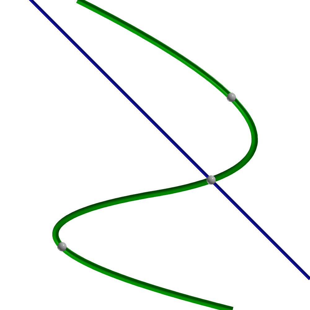
FIGURE: Computes the locations on the freeform curve with local extreme distance to the given line, using CRVLNDST.
CRVPTDST
 NumericType CRVPTDST( CurveType Crv, PointType Point, NumericType IsMinDist,
                       NumericType Epsilon, NumericType Cache )

 or

 ListType CRVPTDST( CurveType Crv, PointType Point, NumericType IsMinDist,
                    NumericType Epsilon, NumericType Cache )
compute the closest (if IsMinDist is TRUE, farthest if FALSE) point on Crv to Point. Since this operation is partially numeric, Epsilon is used to set the needed accuracy. It returns the parameter value of the location on Crv closest to Point. If, however, Epsilon is negative, -Epsilon is used instead, and all local extrema in the distance function are returned as a list (both minima and maxima). If Cache is 1, a cache of precomputed data is prepared following by many point distance evaluations for the SAME CURVE with Cache = 0 that take advantage of this caching, only to terminate and free the cache, when Cache = 2. Cache = 0 should also used when no cache is required.
Example:
Param = CRVPTDST( Crv, Pt, FALSE, 0.0001, 0 );
finds the farthest point on Crv from point Pt. See figure for an example.
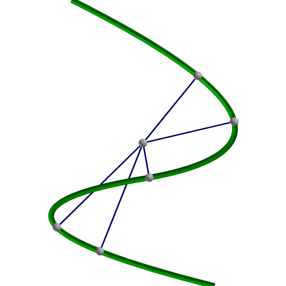
FIGURE: Computes the locations on the freeform curve with local extreme distance to the given point, using CRVPTDST.
CRVPTTAN
ListType CRVPTTAN( CurveType Crv, PointType Pt, NumericType FineNess )
computes all the tangents to Crv that go through point Pt, all in the XY plane. A list of points with X and Y coefficients representing the parametric locations on Crv of the bi-tangent is returned. FineNess controls the numerical accuracy of the computation. A value of 0.01 will provide a good start, and the smaller this number is, the better the accuracy will be. See also CRV2TANS and CNVXHULL.
Example:
    Tans = nil();
    Pt = point( 2, 0, 0 );
    CrvPtTns = CrvPtTan( Crv, Pt, 0.01 );
    for ( i = 1, 1, sizeof( CrvPtTns ),
        snoc( ceval( Crv, nth( CrvPtTns, i ) ) + coerce( Pt, e3 ), Tans ) );
finds the tangents of Crv through Pt and converts them to a set of line segments. See figure for an example.
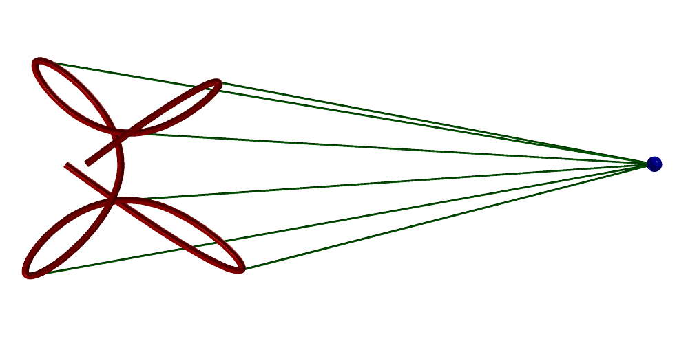
FIGURE: Computes the tangents of a freeform curve through a point, using CRVPTTAN.
CSINE
 CurveType CSINE( NumericType NumCycles, NumericType Samples,
                  NumericType CtlPtsPerVCycle )
constructs a polynomial approximation of a sine wave planar curve of NumCycles cycles. The curve is approximated as a least sqaures fit of Samples samples and CtlPtsPerVCycle control points per loop.
Example:
SineW = csine( 3, 100, 16 );
See figure for this sine of 3 loops.
FIGURE: Approximates a sine wave curve using CSINE.
See also CHELIX, CSPIRAL
CSPIRAL
 CurveType CSPIRAL( NumericType NumLoops, NumericType Pitch,
                    NumericType Samples, NumericType CtlPtsPerLoop )
constructs a polynomial approximation of a spiral planar curve of NumLoops loops and specified Pitch. The curve is approximated as a least sqaures fit of Samples samples and CtlPtsPerLoop control points per loop.
Example:
Spiral = cspiral( 5, 0.7, 500, 6 );
See figure for an example.=See figure for this spiral of 5 loops.
FIGURE: Approximates a spiral curve using CSPIRAL.
See also CHELIX, CSIN
CSURFACE
 CurveType CSURFACE( SurfaceType Srf, ConstantType Direction,
                                                          NumericType Param )

 or

 CurveType CSURFACE( TrimSrfType Srf, ConstantType Direction,
                                                          NumericType Param )

 or

 CurveType CSURFACE( TriSrfType Srf, ConstantType Direction,
                                                          NumericType Param )
extract an isoparametric curve out of Srf in the specified Direction (ROW or COL (or DEPTH for triangular surface) at the specified parameter value Param. Param must be contained in the parametric domain of Srf in Direction direction. The returned curve is in the surface Srf. if Srf isa trimmed surface, the trimming informatin is ignored and a full isoparametric curve is returned regardless.
Example:
Crv = CSURFACE( Srf, COL, 0.45 );
extracts an isoparametric curve in the COLumn direction at the parameter value of 0.15 from surface Srf. See also CMESH, COMPOSE, FFKNTLNS, STRIVAR, and MFROMMV. See figure for an example.
FIGURE: Extracts an isoparametric curve from the given surface, using CSURFACE.
CSRFPROJ
 ListType CSRFPROJ( CurveType Crv, SurfaceType Srf,
                    NumericType Tol, NumericType ProjType )

 or

 ListType CSRFPROJ( CurveType Crv, TrimSrfType TSrf,
                    NumericType Tol, NumericType ProjType )
Computes the orthogonal project of 3-space curve CRv onto 3-space surface Srf or trimmed surface TSrf, to within tolerance Tol. ProjType can be one of:
| ProjType | Description |
|---|---|
| 0 | assumes the curve is not on surface and return the projected |
| curve in the surface's parametric domain. | |
| 1 | assumes the curve is not on surface and return the projected |
| curve in Euclidean space. | |
| 20 | assumes the curve is on the surface (or very close) and |
| returns projected curve in surface parametric domain, by | |
| projecting curve sampled points in Srf. | |
| 21 | same as 20 but employs incremental numeric tracing along |
| the proejcted curve, to speed up the computation. | |
| 3 | assumes the curve is on the surface (or very close) and |
| returns projected curve in surface parametric domain, | |
| by solving for zeros in the derivatives of the distance | |
| field with respect to the surface parameters. | |
| 412/413/423 | assumes the curve is on the surface (or very close) and |
| returns projected curve in surface parametric domain | |
| by solving zeros of distance field in XY if 412, in XZ | |
| if 413, and YZ if 423. | |
| 4123 | assumes the curve is on the surface (or very close) and |
| returns projected curve in surface parametric domain | |
| by solving zeros of distance field in XYZ, using three | |
| equations in the subdivision stage, only XY distance in | |
| the numeric stage. |
ProjCrvs = CSRFPROJ( Crv, Srf, 1e-2, 1 );
Computes the projection of Crv onto Srf and return the result in Euclidean space. Note this projection is not one-to-one and hence several disjoint curves may result. See figure for an example.
FIGURE: Projects a 3-space curve (in red) on the given surface, using CSRFPROJ. Four disjoint compoenets result in this case.
CTANGENT
VectorType CTANGENT( CurveType Curve, NumericType Param, NumericType Normalize )
computes the tangent vector to the Curve at the parameter value Param. The returned vector will have a unit length, if Normalize is TRUE.
Example:
Tang = CTANGENT( Crv, 0.5, true );
computes the unit tangent vector to Crv at the parameter value of 0.5. See also CNORMAL, CNRMLCRV.
CTLPT
CPt = CTLPT( ConstantType PtType, NumericType Coord1, ... )
constructs a single control point to be used in the construction of curves and surfaces. Points can have from one to five dimensions, and may be either Euclidean or Projective (rational). Point type is set via the constants E1 to E9 and P1 to P9. The coordinates of the point are specified in order; weight is first if rational.
Examples:
    CPt1 = CTLPT( E3, 0.0, 0.0, 0.0 );
    CPt2 = CTLPT( P2, 0.707, 0.707, 0.707 );
constructs an E3 point at the origin and a P2 rational point with a weight of 0.707. The Projective Pi points are specified as CTLPT(Pn, W, W X1, ... , W Xn).
CTRIMSRF
ListType CTRIMSRF( TrimSrfType TSrf, NumericType Parametric )
extracts the trimming curves of a trimmed surface TSrf. If Parametric is not zero, then the trimming curves are extracted as parametric space curves of TSrf. Otherwise, the trimming curves are evaluated into Euclidean space as curves on the surface TSrf.
Example:
TrimCrvs = CTRIMSRF( TrimSrf, FALSE );
extracts the trimming curves of TrimSrf as Euclidean curves on TrimSrf. See figure for an example.

FIGURE: Extracts the trimming curves in Euclidean space (middle) and parametric space (right) of a trimmed surface (left), using CTRIMSRF.
See also STRIMSRF.
CTRLCYCLE
 ListType CTRLCYCLE( CurveType Crv, NumericType CycleLength,
                     NumericType SubdivTol, NumericType NumericTol )
Computes a control cycle of the given CycleLength around the given control Crv. Solution is computed by mapping the problem to an algebraic set of constraints. See MZERO for the meaning of SubdivTol and NumericTol.
Example:
CyclePts = CTRLCYCLE( CtrlCrv, 3, 0.001, 1e-8 );
computes a cycle of length 3 to curve CtrlCrv. See figure for an example.
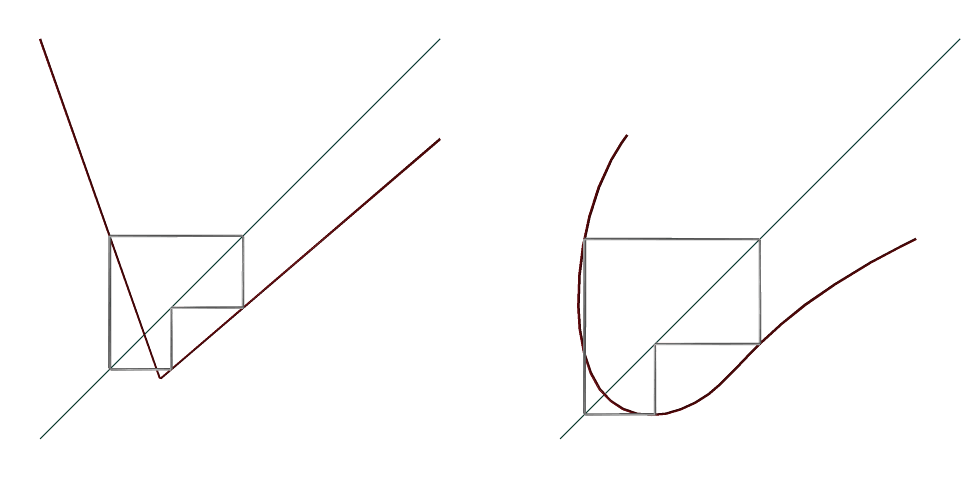
FIGURE: Cycles of length three (in black) to a linear control curve (left) and a cubic control curve (right), computed using CTRLCYCLE.
CMESH
CUBICCRVS
ListType CUBICCRVS( CurveType Crv, NumericType Tolerance, NumericType MaxLen )
approximates given curve Crv using piecewise cubic curves upto the prescribed tolerance Tolerance. If MaxLen is positive it is used to limit the arc length of the cubic curves' segments.
Example:
PCubicCrvs = CUBICCRVS( Crv, 0.01, 0.5 );
creates a piecewise cubic approximation to curve Crv upto tolerance 0.01 and maximal arc length of cubic segments of 0.5. See also QUADCRVS, CBIARCS, and CCUBICS.
CVIEWMAP
 PolygonType CVIEWMAP( CurveType Crv, CurveType ViewCrv,
                       NumericType SubdivTol, NumericType NumerTol,
                       NumericType TrimInvisible )
computes algebraic constraints that reflects the visible domain of planar curve Crv as seen from direction prescribed by planar vector curve ViewCrv. ViewCrv is typically a unit circle curve, parametrizing all possible (360 degrees) planar views. See MZERO for the meaning of the SubdivTol and NumerTol tolerances. If TrimInvisible is FALSE, the return set prescribes the 2D silhouette locations on Crv from the specific view direction. If TrimInvisible is TRUE, attempt ismade to remove the invisile portions. Result is returned as 3D polylines, in (t, v, r) space where t and r parametrize Crv and v parametrizes ViewCrv. This, since a silhouette point Crv(t) could hide a independent curve location Crv(r).
Example:
ViewMap = CVIEWMAP( Crv, pcircle( vector( 0, 0, 0 ), 1 ), 0.1, 1e-6, 0 );
See also CANGLEMAP, CVISIBLE, CARRANGMNT.
CVISIBLE
 PolygonType CVIVISIBLE( CurveType Crv, PointType Pt, NumericType Eps )

 or

 PolygonType CVIVISIBLE( CurveType Crv, VectorType Dir, NumericType Eps )
computes the visible regions of planar curve Crv as seen from either view point Pt or from view direction Dir. Eps controls the accuracy of the computation. Dir must have its Z components zero, whereas Pt's Z coefficient must be one.
Example:
Crvs = CVISIBLE( c, Pt, 1e-5 );
See figure for an example.

FIGURE: The visibility of the given curve on the left is sampled along its 360 degrees to create a visibility atlas of the curve on the right, using CVISIBLE. Then SETCOVER is used to find the minimal set that can see the entire curve, esselntially solving the so-called art-gallery problem.
See also CANGLEMAP, CVIEWMAP, CARRANGMNT, SETCOVER.
CYLIN
 PolygonType CYLIN( VectorType Center, VectorType Direction,
                    NumericType Radius, NumericType Caps )
creates a CYLINder geometric object, defined by Center as the center of the base of the CYLINder, Direction as the CYLINder's axis and height, and Radius as the radius of the base of the CYLINder. If Caps equals zero, no caps are created. If Caps equal one (two), only the bottom (top) cap is created. If Caps equal three, both the top and the bottom caps are created.
See RESOLUTION for the accuracy of the CYLINder approximation as a polygonal model. See IRITSTATE's "PrimRatSrfs" and "PrimRatSrfs" state variables.
Example:
Cylinder1 = CYLIN( vector( 0, 0, 0 ), vector( 1, 0, 0 ), 10, 3 );
constructs a cylinder with two caps of radius 10 along the X axis from the origin to X = 1. See figure for an example.
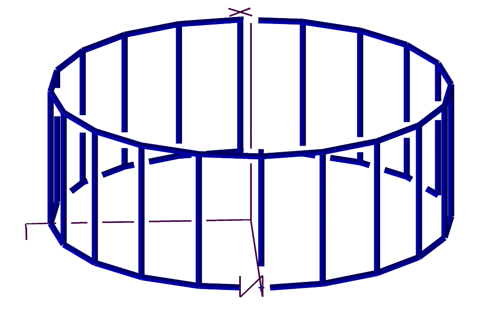
FIGURE: A cylinder primitive can be constructed using the CYLIN constructor.
CZEROS
ListType CZEROS( CurveType Crv, NumericType Epsilon, NumericType Axis )
computes the zero set of the given Crv in the given axis (1 for X, 2 for Y, 3 for Z). Since this computation is numeric, an Epsilon is also required to specify the desired tolerance. It returns a list of all the parameter values (NumericType) the curve is zero.
Example:
    xzeros = CZEROS( cb, 0.001, 1 );
    pt_xzeros = nil();
    pt = nil();
    for ( i = 1, 1, sizeof( xzeros ),
            pt = ceval( cb, nth( xzeros, i ) ):
            snoc( pt, pt_xzeros )
        );
    interact( list( axes, cb, pt_xzeros ), 0 );
computes the X zero set of curve cb with error tolerance of 0.001. This set is then scanned in a loop and evaluated to the curve's locations, which are then displayed. See also CINFLECT. See figure for an example.
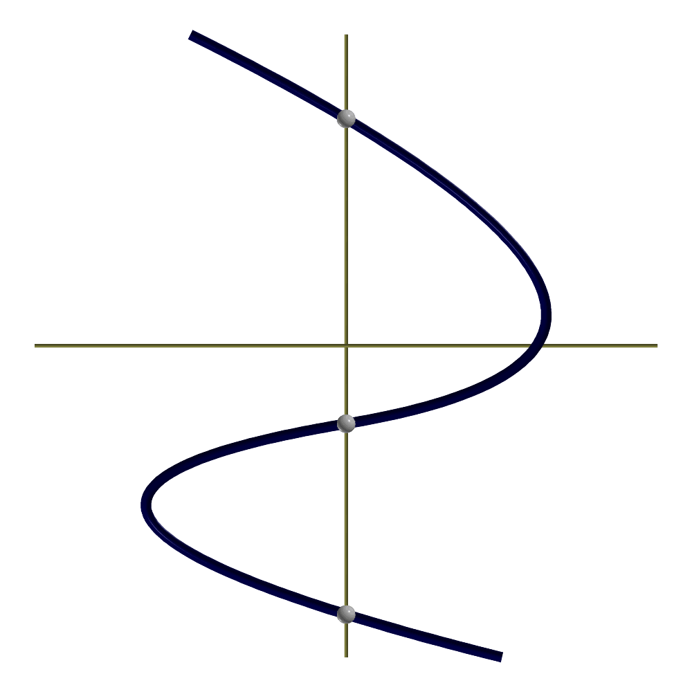
FIGURE: Computes the zero set of a given freeform curve, in the given axis, using CZEROS.
DEPTHPEEL
DEPTHPEEL( AnyType PolyObj, StringType Path, RealType Tesselate )
Peels the depth layers of some polygonal object PolyObj and outputs the sequence of images in path. if Tesselate is set to TRUE, outputs a tesselation of the depth layers. otherwise outputs the number of layers.
 # Output buffer size.
 attrib( Polygonal, "resolution", "1280 x 720" );
 # The near-far tolerance, keep it small, prevents minor clipping.
 attrib( Polygonal, "epsilon", 1e-4 );
 # The XY domain.
 # attrib( Polygonal, "DmnBBox", "(-1, -1)x(1, 1)" );
 DepthPeel( Polygonal, "out.png", TRUE );
Peels Polygonal using the provided parameters and outputs into out0.png, out1.png, ...., outN.png additionally returns a polygonal object that contains the tesselation of all layres.
DIST2FF
 SurfaceType DIST2FF( CurveType Crv1, CurveType Crv2, NumericType DistType )

 or

 MultivarType DIST2FF( CurveType Crv1, SurfaceType Srf2, NumericType DistType )

 or

 MultivarType DIST2FF( SurfaceType Srf1, SurfaceType Srf2, NumericType DistType )
computes the distance function between the two given freeform shapes. The returned variety is bi-variate, tri-variate, or a four-variate, depending on the dimensionality of the input, in order. Based on DistType, the following distance functions could be used:
| DistType Value | Description |
|---|---|
| 0 | Computes the distance vector function, (V1 - V2). |
| 1 | Computes the distance square function, (V1 - V2)^2. |
| 2 | Projection of the distance vector onto the normal |
| field of the first varietly, < V1 - V2, N1 >. | |
| 3 | Projection of the distance vector onto the normal |
| field of the second varietly, < V1 - V2, N2 >. |
Example:
    Crv1 = cbezier( list( ctlpt( E1, .2 ),
                          ctlpt( E2, 0.5, 4 ),
                          ctlpt( E2, 1.3, 0.05 ) ) ) * sy( 0.2 );
    Crv2 = cbezier( list( ctlpt( E1, -.2 ),
                          ctlpt( E2, 0.25, 1.9 ),
                          ctlpt( E2, 1.3, 0.05 ) ) ) * ty( 0.3 ) * sx( 1.5 );
    bb = bbox( dist2ff( Crv1, Crv2, 1 ) );
computes a bound on the minimal and maximal distance square between the given two curves, by computing a bounding box on this scalar distance square field.
DITHERWIRE
 PolyType DitherWire( NumericType Method,
                      StringType Img1, StringType Img2,
                      StringType Proj1, StringType Proj2,
                      ListType Parameters )
Constructs a 3D, wires only, dithering that looks like Img1 from one view direction and like Img2 from another view direction and saves the projections in Proj1 and Proj2 as images.
Method controls the dithering approach as:
1 - Combinatorial, where in iteration, it goes through all possible line in space (between pins on the edges of the cube) and chooses the best one. Grey level. VERY slow.
2 - Combinatorial version of 1 but Colored. VERY slow.
3 - Stochastic, when in iteration, randomly generates N lines and picks the best. Lines spanned an entire cube. Grey level.
4 - Stochastic unbound (meaning that line segments will lay inside a cube). Grey level.
5 - Stochastic, when in iteration, randomly generates N lines and picks the best. Lines spanned an entire cube. Colored.
6 - Stochastic unbound (meaning that line segments will lay inside a cube). Colored. Parameters is a list containing numerical parameters for the dithering method as follows: 1. number of lines to draw, 2. number of pins (relevant for combinatorial methods only), 3. line intensity, 4. weight of feature importance (score multiplier for pixels that lay on edges), 5. Weight of the first image, 6. Weight of the second image, {optional 7. Number of random trials per wire, in stochastic methods}). Returned is a list of 3D lines (and the image projections are asved in Proj1/Proj2.
Example:
   Lines = DitherWire( 3, "image1.png", "image2.png,
                       "projection1.png", "projection2.png",
                       list( 4500, 0, 0.04, 3, 1, 1 ) );
Creates 3D wire dithering with 4500 lines, using stochastic grey level method, and equal weights to both input images. See figure for an example.
FIGURE: An examples of dithering two images simultaneously by 3D wires, using the DITHERWIRE function.
See also DITHERIMAGE and DTRBYCRVS.
DTRBYCRVS
 CurveType DTRBYCRVS( ListType ImageNames, StringType CrvDBFileName,
                      NumericType FloydStein, NumericType Noise,
                      NumericType MergeRows, NumericType DiskShape  )
creates a 3D model cosisting of 3-space curves that dithers two or three images from two or three different view directions. Each curve will serve as a multi directional voxel in 3-space. ImageNames privides a list of two or three image file names. CrvDBFileName specifies a file name that holds a data base of different curves that creates different shading levels from different directions. FloydStein is TRUE to employ Floyd Steinberg error diffusion, or FALSE to ignore. Noise a positive value will add white noise to the images, or zero to disable. If MergeRows is TRUE, all curves in one row will be merged into one object. If FALSE, all curves will reside as individual objects. If DiskShape is TRUE, the created model will be in a disk, or, if FALSE, in a square.
Example:
  CrvMdl = DTRBYCRVS( list( "data/Herzel80.ppm",
                            "data/BenGurion80.ppm" ),
                      "data/DB10x10.itd", TRUE, 0.1, FALSE, FALSE );
creates a model of space curves that dithers the two given PPM images from two views, using the data base DB10x10.itd. Floyd Steinberg is used, some noise (0.1) is added and no rows are merged in the square model that is created. See figure for an example.

FIGURE: An examples of dithering two images simultaneously by 3D wires, using the DTRBYCRVS function.
See also DITHERIMAGE and DTRBYCRVS.
DUALITY
 CurveType DUALITY( CurveType Curve )

 or

 SurfaceType DUALITY( SurfaceType Srf )
computes the dual curve/surface to the given curve/surface. The dual shape is a mapping of every point to a line (plane) in R2 (R3).
Example:
    Ellipsoid = sphereSrf( 1.1 ) * sx( 2 ) * sy( 1.2 );
    DualEllip = DUALITY( Ellipsoid );
See figure for an example.
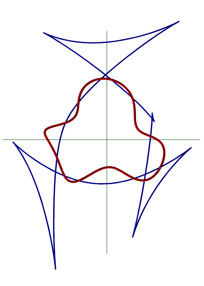
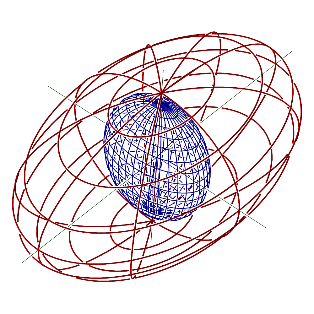
FIGURE: Two examples of a dual curve (left) and a dual surface (right) computed using the DUALITY function. The duals are shown in thin black color.
DVLPSTRIP
 SurfaceType DVLPSTRIP( PointType Pos1, VectorType Tan1, VectorType Nrml1,
                        PointType Pos2, VectorType Tan2, VectorType Nrml2,
                        NumericType OtherScale, NumericType Tension,
                        NumericType DOFs )
computes a developable surface betweek two orientation frames, (Posi, Tani, Nrmli), i = 1, 2. OtherScale controls the other parametrization direction scale where as Tension control the tightness of the shape between the two frame. DOFs controls the number of degrees of freedom (positive value) in the approximated shape or zero to disable additional degrees of freedom.
Example:
DvlpStrip( Pos1, Tan1, Nrml1, Pos2, Tan2, Nrml2, 0.01, 2, 0 );
See also SDVLPCRV, PRISA and PRULEDALG
ELLIPSE3PT
 ListType ELLIPSE3PT( PointType Pt1, PointType Pt2, PointType Pt3,
                      NumericType Offset )
computes the 6 coefficients A-F of,
Ax^2 + Bxy + Cy^2 + Dx + Ey + F = 0,defining the ellipse of minimal area that bounds these 3 points Pti. computation is conducted in the XY plane, with Z ignored. If Offset is not zero, the ellipse is offset approximated by Offset amount.
Example:
    Pt1 = point( random( -0.5, 0.5 ),  random( -0.5, 0.5 ),  0 );
    Pt2 = point( random( -0.5, 0.5 ),  random( -0.5, 0.5 ),  0 );
    Pt3 = point( random( -0.5, 0.5 ),  random( -0.5, 0.5 ),  0 );

    EllImp = ELLIPSE3PT( Pt1, Pt2, Pt3, 0 );
    Ell = ConicSec( EllImp, 0, off, off );
    color( Ell, yellow );
    adwidth( Ell, 2 );
creates three random points in the XY plane and compute the implicit minimal area ellipse for these three points. the Ellipse is realized geometrically using the ConicSec function. See also CONICSEC, IMPLCTTRANS, QUADRIC, MAP3PT2EQL.
EUCOFSTONSRF
 CurveType EUCOFSTONSRF( CurveType Crv, NumericType IsUVCrv, SurfaceType Srf,
                         NumericType OfstDist, NumericType StepTol,
                         NumericType SubdivTol, NumericType NumerTol,
                         NumericType Orient, NumericType TrimOfst,
                         NumericType LSFit )
computes offset approximation to Crv on Srf by offset distance OfstDist. If IsUVCrv TRUE, Crv is assumed a curve in the UVspace of Srf. Otherwise, Crv is assumed in the Euclidean space. StepTol, SubdivTol, and NumerTol control the tolerances of the multivariate solver (see MZERO). Orient can be either -1 or +1, hinting on the desired offset on the left or right of Crv, or 0 to seek both offsets. If TrimOfst TRUE, self intersections in the offset are trimmed away. Finally, LSFit, if not zero, also applies a least square fit with this many control points to get an LS approximation of the result.
    c = pcircle( vector( 0, 0, 0 ), 1 );

    s = surfPRev( cregion( c, 1.3, 2.7 ) * rx( 90 ) );

    cs = compose( s, c, true );

    OfstCrv = EucOfstOnSrf( cs, FALSE, s, 0.2, 0.1, 0.1,
                            1e-10, 0, FALSE, 50 ) );
See figure for an example.
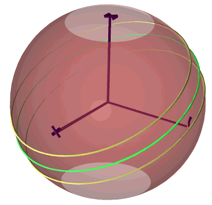
FIGURE: Offset approximation (in dark yellow) of a freeform curve (in green) over a freeform surface, computed using EUCOFSTONSRF.
See also EUCSPRLONSRF.
EUCSPRLONSRF
 CurveType EUCSPRLONSRF( SurfaceType Srf, NumericType Dir,
                         NumericType Pitch, NumericType StepTol,
                         NumericType SubdivTol, NumericType NumerTol,
                         NumericType OutputType )
computes a spiral approximation curve on Srf in Dir (U or V), spiraling by amount Pitch between one spiral to the next. Note Srf isexpected to be closed in the other direction as each spiral must be connected to the next (via the closed boundary). StepTol, SubdivTol, and NumerTol control the tolerances of the multivariate solver (see MZERO). Finally, OutputType can be either 0 for UVT parameteric space output, 1 for curves in Euclidean space, or 2 for merged curves in Euclidean space (adjacent spiral that are continuous are merged).
SpiralCrv = EucSprlOnSrf( s2, col, 0.5, 0.02, 0.01, 1e-10, 2 );
See figure for an example.
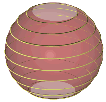
FIGURE: Spiral covering curve approximation over a freeform surface, computed using EUCSPRLONSRF.
See also EUCOFSTONSRF.
EVOLUTE
 CurveType EVOLUTE( CurveType Curve )

 or

 SurfaceType EVOLUTE( SurfaceType Srf )
compute the evolute of a curve or a surface. For curves, the evolute is defined as,
N(t)
E(t) = C(t) + ----
k(t)
where N(t) is the unit normal of C(t), and k(t) is its curvature.
E(t) is computed symbolically as the symbolic sum of C(t) and
N(t) / k(t).For surfaces, this function computes the mean evolute which is equal to,
n(u, v)
E(u, v) = S(u, v) + ---------
2 H(u, v)
where n(u, v) is the unit normal of S(u, v), and H(u, v) is its mean
curvature. E(u, v) is computed symbolically.
The result of this symbolic computation is exact (upto machine precision), unlike similar operations such as OFFSET or AOFFSET, that are only approximated.
Example:
    crv = cbspline( 3,
                    list( ctlpt( E3, -1.0,  0.1,  0.2 ),
                          ctlpt( E3, -0.1,  1.0,  0.1 ),
                          ctlpt( E3,  0.1,  0.1,  1.0 ),
                          ctlpt( E3,  1.0,  0.1,  0.1 ),
                          ctlpt( E3,  0.1,  1.0,  0.2 ) ),
                    list( KV_OPEN ) );
    cev = EVOLUTE( Crv );
See figure for an example.
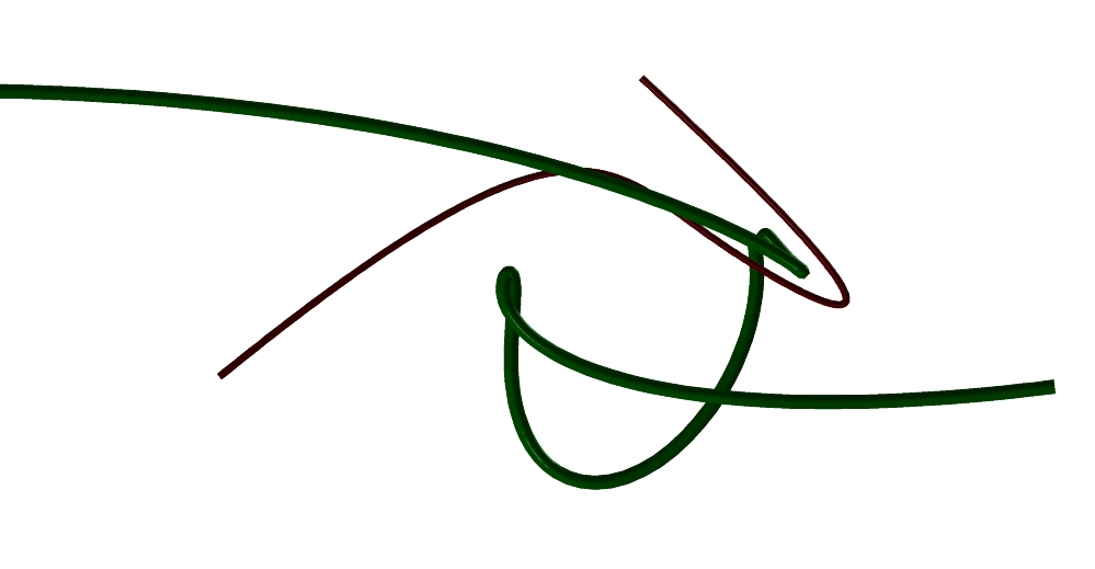
FIGURE: The evolute (thick) of a freeform curve (thin) can be computed using EVOLUTE.
See also SMEAN.
EXPLODE
ListType EXPLODE( ListType Object, NumericType ExpType, VectorType ExpCenter,
NumericType ExpAmount, VectorType ExpDir,
NumericType AnimCrvs )
@end{verbatim}
Translates the elements of a given list object geometry {bf Object} in
different directions: spherically from ExpCenter if {ExpType} is
FALSE, or cylindrically along ExpDir if TRUE. The amount of
the explosion is governed by ExpAmount. Only the top level elements
of list geometry Object are affected by this function. If
AnimCrvs is TRUE, animation curves are added to Object, or
if FALSE, transformation matrices.
Example:
GeomExp = EXPLODE( Geom, FALSE, vector( 0, 0, 0 ), 0.35,
vector( 0, 0, 0 ), FALSE );
Radially (spherically) explodes all sub-elements in list object Geom,
around the origin.
EXTRUDE
PolygonType EXTRUDE( PolygonType Object, VectorType Dir, NumericType Caps )
or
SurfaceType EXTRUDE( CurveType Object, VectorType Dir, NumericType Caps )
or
VModelType EXTRUDE( TrimSrfType Object, VectorType Dir, NumericType Caps )
or
TrivarType EXTRUDE( SurfaceType Object, VectorType Dir, NumericType Caps )
or
TrivarType EXTRUDE( ListType Object, VectorType Dir, NumericType Caps )
Creates an extrusion of the given Object. If the Object is a
PolygonObject, its first polygon is used as the base for the extrusion in
Dir direction. If the Object is a CurveType, an extrusion surface is
constructed. If the Object is a SurfaceType, an extrusion trivariate
is constructed. If the Object is a TrimSrfType, an extrusion VModelType
is constructed. If the Object is a ListType, a list of extruded objects
is created for the objects found in Object.
If Caps equals zero, no caps are created. If Caps equal one
(two), only the bottom (top) cap is created. If Caps equal three,
both the top and the bottom caps are created.
Note that caps are created for a closed Object only, so the Object
must be either a polygon or a closed curve for caps to be generated.
Direction Dir cannot be coplanar with the polygon plane. The curve
may be nonplanar.
Example:
Cross = cbspline( 3,
list( ctlpt( E2, -0.018, 0.001 ),
ctlpt( E2, 0.018, 0.001 ),
ctlpt( E2, 0.019, 0.002 ),
ctlpt( E2, 0.018, 0.004 ),
ctlpt( E2, -0.018, 0.004 ),
ctlpt( E2, -0.019, 0.001 ) ),
list( KV_OPEN ) );
Cross = Cross + -Cross * scale( vector( 1, -1, 1 ) );
Napkin = EXTRUDE( Cross * scale( vector( 1.6, 1.6, 1.6 ) ),
vector( 0.02, 0.03, 0.2 ),
0 );
constructs a closed cross section Cross by duplicating one half of
it in reverse and merging the two sub-curves. Cross is then used as
the cross section for the extrusion operation.
See figure for an example.
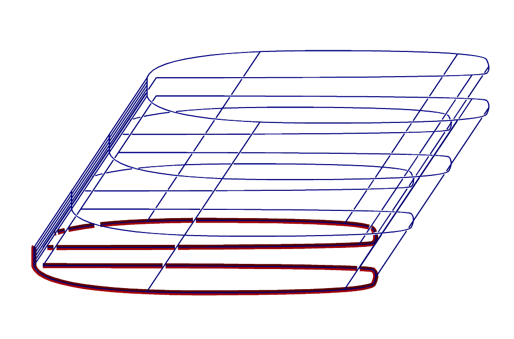
FIGURE:
An extrusion of a freeform curve using EXTRUDE to create a freeform
surface.
See also ZTEXTRUDE, RULEDSRF, RULEDTV, and RULEDVMDL.
FFCMPCRVS
FFCMPCRVS( CurveType Crv1, CurveType Crv2, NumericType Tolerance )
compares the given two curves, Crv1 and Crv2 for an
identical trace. Curves could have identical trace while with
different degrees (via degree raising of one of them), differet knot
sequences (by applying refinements to either curves or both), or even
different speed (via composition). This function reduces both curves
to a canonical representation by reverse engineering unnecessary
degree raising, refinements, or composition and then compare the two
curves upto the given tolerance Tolerance.
Returned is a list of 5 numeric values. The first number equals 1
if the curves are the same, 2 if the are the same but domain is not
exactly the same, or 3 f the curves are different. The other four numbers
in the list are the domains of the two given curves that overlap as
(Start1, End1, Start2, End2).
Example:
Similarity = FFCMPCRVS( Crv1, Crv2, 1e-6 );
FFCOMPAT
FFCOMPAT( CurveType Crv1, CurveType Crv2 )
or
FFCOMPAT( SurfaceType Srf1, SurfaceType Srf2 )
make the given two curves or surfaces compatible by making them share
the same point type, the same curve type, the same degree, and the
same continuity. The same point type is gained by promoting a lower
dimension into a higher one, and non-rational to rational
points. Bezier curves are promoted to B-spline curves if necessary,
for curve type compatibility. Degree compatibility is achieved by
raising the degree of the lower order curve. Continuity is achieved
by refining both curves to the space with the same (unioned) knot
vector. This function returns nothing and compatibility is made in place}.
Example:
FFCOMPAT( Srf1, Srf2 );
See also CMORPH and SMORPH.
FFCTLPTS
ListType FFCTLPTS( FreeformType Freeform );
returns all the control points of the given Freeform in a single list.
See Also FFPTTYPE, FFGTYPE, FFKNTVEC, FFMSIZE, FFORDER.
Example:
Ctls = FFCTLPTS( Srf1 );
FFEXTEND
CurveType FFEXTEND( CurveType Crv, ListType Ends, ListType ExtendEps,
Numeric RemoveExtraKnots )
or
SurfaceType FFEXTEND( SurfaceType Srf, ListType Ends, ListType ExtendEps,
Numeric RemoveExtraKnots )
or
TrivarType FFEXTEND( TrivarType TV, ListType Ends, ListType ExtendEps,
Numeric RemoveExtraKnots )
or
MultivarType FFEXTEND( MultivarType MV, ListType Ends, ListType ExtendEps,
Numeric RemoveExtraKnots )
If a Crv, extends the given Crv in either one of its two ends
as is specified by the list Ends of two Booleans parameters, an amount
equals to ExtendEps.
If a Srf, extends the given Srf in either one of its four sides
as is specified by the list Ends of four Booleans parameters, an amount
equals to ExtendEps.
If a TV, extends the given TV in either one of its six faces
as is specified by the list Ends of six Booleans parameters, an amount
equals to ExtendEps.
If an MV, extends the given MV of dimension n, in either one of
its 2n faces as is specified by the list Ends of 2n Booleans parameters,
an amount equals to ExtendEps.
If RemoveExtraKnots is true redundant knots are removed.
The extension is computed so that the new entity will preserve the original
domain and hence will be identical for the original domain, to the input.
In all cases, an "ExtntScl" attribute with a factor different than one can
be placed on the geometry in whcih case the extended geometry will be scaled
following thsi factor. When relevant (surfaces and trivariates), also
"ExtntSclU", "ExtntSclV", and "ExtntSclW" can be used to affect the scale in
that direction. Note that scaling the extension will also affect the size
(number of control points) of the resulting geometry.
Example:
C1ext = FFEXTEND( c1, list( true, true ), list( 0.1 ), true );
extends curve c1 at both its ends by 0.1.
FFEXTREMA
ListType FFEXTREMA( CurveType Crv, NumericType Euclidean )
or
ListType FFEXTREMA( SurfaceType Srf, NumericType Euclidean )
or
ListType FFEXTREMA( trivarType TV, NumericType Euclidean )
computes and returns the parameter locations of local extrema values of
given scalar freeform (a curve, surface, or trivariate). Returned is a list
of parameter locations where the extreme is taking place (interior location,
boundary location or possibly C^1 discontinuity location.
However, if Euclidean is true, the results are mapped to Euclidean
space.
Example:
Extrema = FFEXTREMA( Srf, false );
computes a list of all parameter locations where Srf assumes local
extrema. See also FFEXTREME
FFEXTREME
CtlPtType FFEXTREME( CurveType Crv, NumericType Minimum )
or
CtlPtType FFEXTREME( SurfaceType Srf, NumericType Minimum )
or
CtlPtType FFEXTREME( trivarType TV, NumericType Minimum )
compute a bound on the extreme values a curves Crv or surface
Srf or trivariate TV can assume. Returned control point
provides a bound on the minimum (maximum) values that can be assumed
if Minimum is TRUE (FALSE).
Example:
Bound = FFEXTREME( Srf, false );
computes a bound on the maximal values Srf can assume. See also
FFEXTREMA
FFGTYPE
NumericType FFGTYPE( FreeformType Freeform )
returns the geometric type (BEZIER_TYPE, BSPLINE_TYPE etc.) of the given
freeform.
See Also FFGTYPE, FFCTLPTS, FFKNTVEC, FFMSIZE, FFORDER, PDOMAIN.
FFKNTLNS
CurveType FFKNTLNS( SurfaceType Srf, NumericType Pllns )
or
PolyType FFKNTLNS( SurfaceType Srf, NumericType Pllns )
returns all isoparametric curves that are at an interior knot of the
surface Srf. If, however, Pllns is true, the result is converted
to a piecewise linear approximation (i.e. polylines).
Example:
KntCrvs = FFKNTLNS( Srf, false );
See also GPOLYLINE, CSURFACE and CMESH.
FFKNTVEC
ListType FFKNTVEC( FreeformType Freeform )
returns all the knot vector(s) of the given Freeform in a list of knot
vector(s). See Also FFPTTYPE, FFGTYPE, FFCTLPTS, FFMSIZE, FFORDER.
Example:
KVs = FFKNTVEC( Srf1 );
FFMATCH
FFMATCH( CurveType Crv1, CurveType Crv2, NumericType Reduce,
NumericType Samples, NumericType ReparamOrder,
NumericType Rotate, NumericType NormType, NumericType MaxError )
computes a reparametrization to Crv2 so it fits Crv1, the best
under some prescribed norm, NormType. Currently the following norms
are valid for NormType
| Value | Description |
|---|---|
| 1 | Suitable for ruled and blended curves, for modeling. |
| See RULEDSRF. | |
| 2 | Suitable for metamorphosis of curves. See CMORPH. |
| 3 | Distance norm in "walking the dog" notion. |
| 4 | Bisector (skeleton) matching norm for two curves. |
| 5 | Another variant for ruled and blended curves, for |
| modeling. See RULEDSRF. |
The reparametrization is computed by sampling a fixed set of size Samples off both curves, and fitting a B-spline curve of length Reduce as the reparametrization curve. Hence, Reduce must be less than or equal to Samples. The reparametrization curve will have order of ReparamOrder. If Rotate is TRUE or ON, then attempt is made to rotate the reparametrization of the curves. Rotation can be used on closed curves only. if MaxError is TRUE the maximal error is minimized. Otherwise, the error's sum over the entire domain is minimized.
See RULEDSRF and CMORPH for examples.
FFMERGE
 CurveType FFMERGE( ListType E1Curves, NumericType PointType )

 or

 SurfaceType FFMERGE( ListType E1Surfaces, NumericType PointType )

 or

 MultivarType FFMERGE( ListType E1Multivars, NumericType PointType )
merge the scalar curves/surfaces/multivariates in the list of curves E1Curves or list of surfaces E1Surfaces or list of multivariates E1Multivars to one vector curve/surface/multivariate of point type PointType.
Example:
Srf = FFMERGE( list( SrfW, SrfX, SrfY ), P2 );
merges three scalar surfaces into a single surface with point type P2. See also FFSPLIT.
FFMESH
ListType FFMESH( FreeformType Freeform )
returns the control mesh/polygon of the given Freeform in a list. See Also FFCTLPTS, FFKNTVEC, FFORDER, FFPTTYPE, FFMSIZE.
Example:
SrfMesh = FFMESH( Srf );
FFMSIZE
ListType FFMSIZE( FreeformType Freeform )
returns the size of the control mesh/polygon of the given freeform in a list. See Also MESHSIZE, FFMESH, FFPTTYPE, FFGTYPE, FFCTLPTS, FFKNTVEC, FFORDER, PDOMAIN.
Example:
MSizes = FFMSIZE( Srf1 );
FFORDER
ListType FFORDER( FreeformType Freeform )
returns all the orders of the given Freeform in a single list. See Also FFPTTYPE, FFGTYPE, FFCTLPTS, FFKNTVEC, FFMSIZE, PDOMAIN.
Example:
Orders = FFORDER( Srf1 );
FFPOLES
NumericType FFPOLES( FreeformType Freeform );
returns TRUE if the given Freeform has poles, FALSE otherwise. Poles are zeros in the weights of rational functions.
Example:
HasPoles = FFPOLES( Srf1 );
See also FFSPLTPOLES
FFPTDIST
 ListType FFPTDIST( CurveType Crv, NumericType Param, NumericType NumOfPts )

 or

 ListType FFPTDIST( SurfaceType Srf, NumericType Param, NumericType NumOfPts )
compute a uniform point distribution for Crv or Srf. If Param is FALSE, the distribution is selected to be uniform in the Euclidean space; otherwise if TRUE, the distribution is made uniform in the parametric space. NumOfPts sets the number of points in the distribution.
The returned list of points prescribes parameter values in the freeforms. For Crv, the returned list is a list of reals, in the parameter space of Crv. For Srf, the returned list is a list of points, whose X and Y coefficients hold the U and V parameters of Srf. See also COVERPT.
Example:
    c1 = cbezier( list( ctlpt( E2, -1.0,  0.0 ),
                        ctlpt( E2, -1.0,  0.1 ),
                        ctlpt( E2, -0.9, -0.1 ),
                        ctlpt( E2,  0.9,  0.0 ) ) );
    color( c1, magenta );

    pts = FFPTDIST( c1, true, 300 );
    e2pts = nil();
    for ( i = 1, 10, sizeof( pts ),
            pt = ceval( c1, coord( nth( pts, i ), 0 ) ):
            snoc( pt, e2pts )
        );
    interact( list( e2pts, c1 ) );

    pts = FFPTDIST( c1, false, 300 );
    e2pts = nil();
    for ( i = 1, 10, sizeof( pts ),
            pt = ceval( c1, coord( nth( pts, i ), 0 ) ):
            snoc( pt, e2pts )
        );
    interact( list( e2pts, c1 ) );
computes the distribution of 100 points in curve c1 which has highly nonuniform speed characteristics. Two distributions are computed, one to be uniform in the parametric space and one to be uniform in the Euclidean space. See figure for an example.
FIGURE: (top) A distribution of 30 points uniformly in Euclidean space. (bottom) A distribution of 30 points uniformly in parameteric space. Both examples were computed using FFPTDIST.
FFPTTYPE
NumericType FFPTTYPE( FreeformType Freeform )
returns the point type (E2, P4 etc.) of the given freeform. See Also FFGTYPE, FFCTLPTS, FFKNTVEC, FFMSIZE, FFORDER, PDOMAIN.
FFSPLIT
 ListType FFSPLIT( CurveType Crv )

 or

 ListType FFSPLIT( SurfaceType Srf )

 or

 ListType FFSPLIT( MultivarType MV )
split the given curve Crv or surface Srf or multivariate MV into its scalar components that are returned as a list of scalar curves/surfaces/multivariates.
Example:
E1Srfs = FFSPLIT( circle( vector( 0, 0, 0 ), 1 ) );
splits the circle which is a curve in P3 into four scalar curves (W, X, Y, Z) that are returned in a single list. See also FFMERGE, FFPTTYPE.
FFSPLTPOLES
 ListType FFSPLTPOLES( CurveType Crv, NumericType SubdivTol,
                       NumericType NumericTol, NumericType Offset,
                       NumericType Option )

 or

 ListType FFSPLTPOLES( SurfaceType Srf, NumericType SubdivTol,
                       NumericType NumericTol, NumericType Offset,
                       NumericType Option )
If Option = 0, the domain locations of the poles, locations were the denominator vanish (points in the case of rational input Crv, curves in the case of rational input Srf), is computed. If Option = 1, splits the given rational Crv or Srf at its poles. In the case of surfaces, the result is a list of trimmed surfaces as the poles are not necessarily isoparameteric. If Offset is not zero, the neighborhood of the pole is clipped as well upto a distance offset in the parametric domain from the pole. If Option = 2, and only in the case of Srf, subdivides the given Srf up to {SubdivTol}, to patches that are poles-free and return only poles-free such patches.
Example:
Crvs = FFSPLTPOLES( crv, 0.01, 1e-10, 0.001, 1 );
See also FFPOLES.
FITPMODEL
 ListType FITPMODEL( PolygonType PlObj, NumericType FitType,
                     NumericType Tol, NumericType NumIters )
fits a primitive object to the given polygonal model, PlObj. The numeric fitting process is controled via a bound on the number of iterations NumIters and the resulting tolerance of the fit that is required, Tol. Returned is a list of numeric values with the error of the fit as the first value. The rest of the list numeric values are the coefficients of the algebraic fitted form (see table below). FitType can be one of:
| 0 | A Planar face. Returned list holds (A, B, C, D), the four |
|---|---|
| coefficients of the plane equation. | |
| 1 | A Sphere. Returned list holds (Xcntr, Ycntr, Zcntr, Radius) |
| of the fitted sphere. | |
| 2 | A Cylinder. Returned list holds (Xcntr, Ycntr, Zcntr, |
| Xdir, Ydir, Zdir, Radius) of the fitted cylinder. | |
| 3 | A Circle. Returned list holds (Xcntr, Ycntr, Radius) of |
| the fitted circle. | |
| 4 | A Cone. Returned list holds (Xcntr, Ycntr, Zcntr, |
| Xdir, Ydir, Zdir, Radius) of the fitted cone. |
Example:
resolution = 20; x1 = triangl( sphere( vector( 1, 2, 3 ), 4 ), 1 ); SprParams = FitPModel( x1, 1, 0.01, 100 );
Computes a fitted sphere to a polygonal approximation of a sphere. See also ANALYFIT.
FINDATTR
ListType FINDATTR( ListType Objs, StringType AttrName, AnyType AttrVal,
NumericType LeavesOnly, NumericType Negate )
Filters only objects in Objs that have attributes named AttrName and value AttrVal. AttrVal can be nil() for filtering only based on AttrName. If LeavesOnly is TRUE, only leaves in the hierZchy of Objs are searched for a match. If Negate is TRUE, only objects that do not have AttrName (and value AttrVal) are considered as matched.
Example:
Mf = FindAttr( M, "BzrIndex", "0,0,3", true, true );
extracts all leave elements in M that have a "BzrIndex" attribute and attribute value "0,0,3".
See also ATTRIB, ATTRPROP, ATTRVPROP, CPATTR, GETATTR.
FIXPLGEOM
PolygonType FIXPLGEOM( PolygonType PlObj, NumericType Oper, NumericType Eps ) or ListType FIXPLGEOM( ListType Obj, NumericType Oper, NumericType Eps )
cleans polygonal geometry. based on Oper, the following will be conducted:
| 0 | Remove identical duplicated polygons. |
|---|---|
| 1 | Remove zero length edges. |
The clean up of an object will be applied individually to each part found in the object list Obj.
Example:
Obj2 = FIXPLGEOM( Obj, 0 ); Obj3 = FIXPLGEOM( Obj2, 1 ); Obj4 = FIXPLNRML( Obj3, 2 );
cleans duplicated polygons, zero length edges, and then reorient the result. See also FIXPLNRML.
FIXPLNRML
PolygonType FIXPLNRML( PolygonType PlObj, NumericType TrustInfo ) or ListType FIXPLNRML( ListType Obj, NumericType TrustInfo )
corrects inconsistencies in polygonal geometry, between normals of polygons and normals at the vertices based on TrustInfo. As a side effect also allow the split of a polygonal models with disjoint parts, into the disjoint parts. That is, every connected component in the input will be returned as a separated object. If TrustInfo is
| 0 | Trust the normals at the vertices. |
|---|---|
| 1 | Trust the normals of the polygons. |
| 2 | Reorient all the polygon's normals and vertices |
| normals to follow the orientation of first polygon. | |
| 3 | Same as 2 but also splits disjoint part in the |
| input object to different objects. |
The computation on an object will be applied individually to each part found in the object list Obj. Option 2 of TrustInfo will correct cases where adjacent polygons are not oriented the same, based on detection of adjacencies.
Example:
Obj2 = FIXPLNRML( Obj, 2 );
See also FIXPLGEOM and SMOOTHNRML.
FLATTENHIER
ListType FLATTENHIER( ListType List )
Flatten a hierachy of objects in a single list object of elements, all of which are leaves.
See also MERGEATTR, MERGELIST, MERGEPOLY, MERGEPLLN, MERGETYPE, SPLITLST.
GBOX
PolygonType GBOX( VectorType Point,
VectorType Dx, VectorType Dy, VectorType Dz )
or
TrivarType GBOX( PointType P000, PointType P001,
PointType P010, PointType P011,
PointType P100, PointType P101,
PointType P110, PointType P111 )
or
TrivarType GBOX( VectorType UMinVec, VectorType UMaxVec,
VectorType VMinVec, VectorType VMaxVec,
VectorType WMinVec, VectorType WMaxVec )
The first form creates a polygonal parallelepiped - a generalized BOX polygonal object, defined by a Point as its base position, and Dx, Dy, Dz as 3 3D vectors to define the 6 faces of this generalized BOX. The regular BOX object is a special case of GBOX where Dx = vector(Dx, 0, 0), Dy = vector(0, Dy, 0), and Dz = vector(0, 0, Dz). Dx, Dy, Dz must all be independent in order to create an object with positive volume.
The second form creates a generalized box trivariate - given the eight corner points of the desired generalized box as Pxxx. The third form also creates a generalized box trivariate - given six desired (not necessarily unit) normals of the six faces of the box, as xMinVec/xMaxVec. Since this third form is in a vector space, the resulting cube is positioned around the origin and in [-1, 1]^3;
Note that in the second and third forms, the faces will not necessarily be planar (and hence the normals requested are only approximated).
Example:
GB = GBOX( vector( 0.0, -0.35, 0.63 ), vector( 0.5, 0.0, 0.5 ),
vector( -0.5, 0.0, 0.5 ),
vector( 0.0, 0.7, 0.0 ) );
See figure for an example.
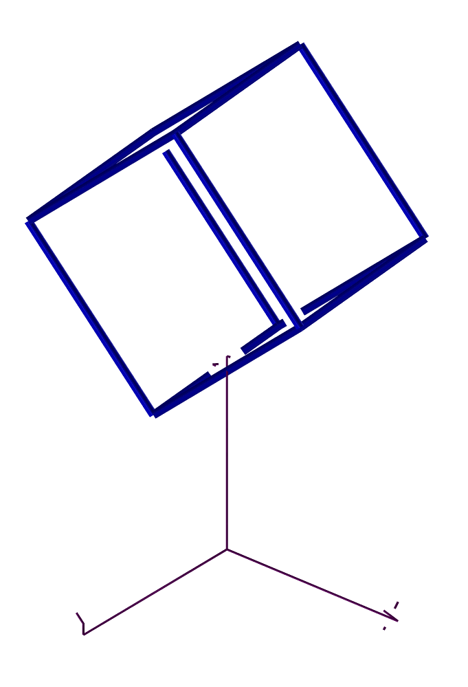
FIGURE: A warped box in a general position can be constructed using the GBOX constructor.
GEAR2DSWEEP
NumericType GEAR2DSWEEP( NumericType FuncType, ListType Params ) or CurveType GEAR2DSWEEP( NumericType FuncType, ListType Params )
computes 2D gears, given a teeth wheel geometry, not necessarily circular. FuncType can be one of
| 1 | To compute the conjugate wheel. Here Params is a |
|---|---|
| list of two parameters (Wheel1Crv, SolverStepSize). | |
| 2 | To arrange teeth. Here Params is a list of |
| three parameters (Wheel2Crv, ToothLength, NumTeeth). | |
| 3 | To derive the centrode. Here Params is a list of |
| two parameters (WheelSurface, SolverStepSize). | |
| 4 | To employ uniform motion in the forecoming gear computations. |
| Here Params is a list of two parameters | |
| (GearDistance, SolverStepSize). | |
| 5 | To employ non uniform motion in the forecoming gear computations. |
| Here Params is a list of three parameters | |
| (GearDistance, SolverStepSize, Wheel1Crv). | |
| 6 | To handle oblong motion in the forecoming gear computations. Here |
| Params is a list of six parameters (GearDistance, ToothLength, | |
| NumTeeth, NumTeethCirc, NumTeethLinear, InverseMotion). | |
| 7 | to derive the inverse motion. |
Gear2DSweep( GEAR2D_UNIFORM_MOTION, list( GearDist, SolverStepSize ) );
CrvH0 = Gear2DSweep( GEAR2D_CONJUGATE, list( CrvG0, SolverStepSize ) );
Gear2DSweep( GEAR2D_UNIFORM_MOTION, list( GearDist, SolverStepSize ) );
CrvG1 = Gear2DSweep( GEAR2D_CONJUGATE, list( CrvH0, SolverStepSize ) );
computes the gear with uniform motio nas the conjugate of the input wheel {bf CrvG0}, as CrvH0, only to derive the conjugate to CrvH0, as CrvG1.
GETATTR
AnyType GETATTR( AnyType Obj, StringType Name )
provides a mechanism to fetch an attribute named Name from object Obj.
Example:
attrib( axes, "test", 15 );
a = GETATTR( axes, "test" );
will set the value of a to be 15.
GETLINE
AnyType GETLINE( NumericType RequestedType )
provides a method to get input from the keyboard within functions and or subroutines. RequestedType can be a NUMERIC_TYPE, E2, POINT_TYPE, VECTOR_TYPE, or PLANE_TYPE in which the entered line will be parsed into one, two, three, or four numeric values (operated by either spaces or commas) and the proper object will be created and returned. RequestedType can also be CTLPT_TYPE in which case as many numeric values in the line are read into an En control point (up to the maximal dimension of a control point). In any other case, including failure to parse the numeric input, a STRING_TYPE object will be constructed from the entered line.
Example:
Pt = GETLINE( point_type );
to read one point (three numeric values) from stdin.
GETNAME
StringType GETNAME( ListType ListObj, NumericType Index )
gets the name of a sub object of index Index in list object ListObj. Index of the first element is one.
Example:
A = list( XX, Second, C );
GETNAME( A, 1 );
returns the name of the second element, "Second".
See also SETNAME.
GGINTER
ListType GGINTER( CurveType Srf1Axis, CurveType Srf1Rad,
CurveType Srf2Aixs, CurveType Srf2Rad,
NumericType SubdivTol, NumericType ZeroSetFunc )
computes the intersection curves of the given two ring surfaces, defined as spine surfaces with axis SrfiAxis, i = 1, 2 and circular cross section along the normal plane of the axis curve with radii SrfiRad.
The ring ring intersection (RRI) problem is tranformed into a zero set finding on another function. If ZeroSetFunc is true, the function whose zero set provides the RRIsolution is returned. Otherwise, if ZeroSetFunc is false, the RRI solution itself is returned. The zero set is computed via numerical zero set finding methods and Tolerance controls the fineness of the approximated solution. See figure for an example.
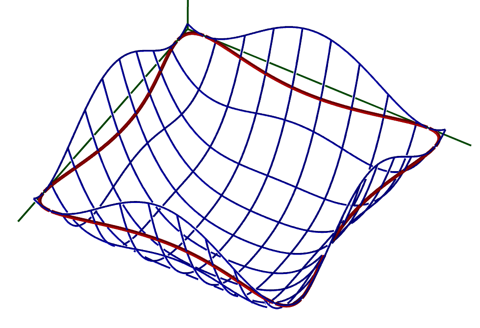
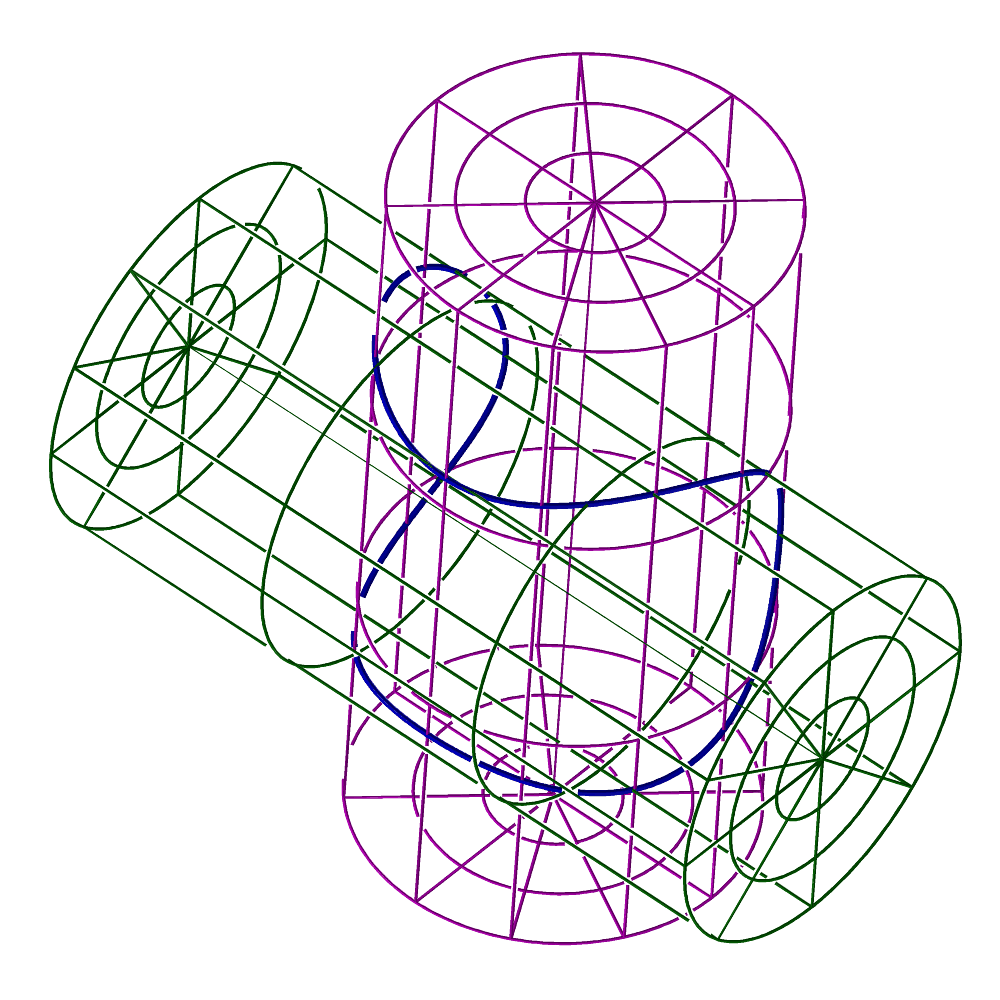
FIGURE: Computation of the intersection curve between two ring surfaces via the GGINTER command. On the left, the zero set function is displayed while on the right, the computed intersection between two ocylinders is shown.
Example:
s1 = cylinSrf( 4, 1 ) * tz( -2 );
c1 = cbezier( list( ctlpt( E3, 0.0, 0.0, -1.0 ),
ctlpt( E3, 0.0, 0.0, 1.0 ) ) );
r1 = cbezier( list( ctlpt( E1, 1.0 ) ) );
s2 = cylinSrf( 4, 1 ) * tz( -2 ) * rx( 90 ) * tx( 0.5 );
c2 = cbezier( list( ctlpt( E3, 0.5, -1.0, 0.0 ),
ctlpt( E3, 0.5, 1.0, 0.0 ) ) );
r2 = cbezier( list( ctlpt( E1, 1.0 ) ) );
ZeroSetSrf = coerce( GGINTER( c1, r1, c2, r2, 0.1, true ), e3 )
* rotx( -90 ) * roty( -90 );
resolution = 100;
ZeroSet = contour( ZeroSetSrf, plane( 0, 0, 1, 0 ) );
interact( list( ZeroSetSrf * sz( 0.1 ), ZeroSet, axes ) );
c = nth( GGINTER( c1, r1, c2, r2, 0.03, false ), 1 );
interact( list( s1, s2, c ) );
constructs two cylinders as s1 and s2, defines the same two cylinders as a ring surface with axes spines of c1 and c2 and a constant radius, one in r1 and r2, and computes the zero set of the intersection and the intersection curve itself. See also RRINTER, SSINTER and SSINTR2.
GPOINTLIST
PolylineType GPOINTLIST( GeometryTreeType Object, NumericType Optimal,
NumericType Merge )
converts all Curves(s), (Trimmed) Surface(s), and Trivariate(s) Object into pointlists using the RESOLUTION variable. The larger the RESOLUTION is, the finer the resulting approximation will be. Returns a single pointlist object if Merge is TRUE.
If Optimal is false, the points are sampled at equally spaced intervals in the parametric space. If Optimal true, a better, more expensive computationally algorithm is used to derive optimal sampling locations so as to minimize the maximal distance between the curve and piecewise linear approximation (L infinity norm).
Example:
Pts = GPOINTLIST( list( Srf1, Srf2, Srf3, list( Crv1, Crv2, Crv3 ) ),
true, true );
See also GPOLYGON, GPOLYLINE.
GPOLYGON
PolygonType GPOLYGON( GeometryTreeType Object, NumericType Normals )
approximates all Surface(s)/Trimmed surface(s)/Trivariate(s) in Object with polygons using the POLY_APPROX_OPT, POLY_APPROX_TRI, POLY_MERGE_COPLANAR, RESOLUTION and FLAT4PLY variables. If POLY_APPROX_OPT is FALSE, RESOLUTION vaguely prescribes the number of uniform (in parametric space) samples to sample the surface in each direction. If POLY_APPROX_OPT is TRUE, POLY_APPROX_TOL prescribes the maximal deviation of the polygonal approximation from the original surface, in object space coordinates. IF POLY_APPROX_TRI is TRUE, only triangles are generated on the output set. POLY_MERGE_COPLANAR controls the way coplanar adjacent polygons are merged into one (or not.) FLAT4PLY is a Boolean flag controlling the conversion of an (almost) flat patch into four (TRUE) or two (FALSE) polygons. Normals are computed to polygon vertices using surface normals, so Gouraud or Phong shading can be exploited. It returns a single polygonal object.
If Normals is set, surface normals will be evaluated at the vertices. Otherwise flat shading and constant normals across polygons are assumed.
Example:
Polys = GPOLYGON( list( Srf1, Srf2, Srf3 ), off );
converts to polygons the three surfaces Srf1, Srf2, and Srf3 with no normals. See also GPOINTLIST, GPOLYLINE, POLY_APPROX_OPT, POLY_APPROX_TOL, POLY_APPROX_TRI, POLY_APPROX_UV, POLY_MERGE_COPLANAR, RESOLUTION and FLAT4PLY.
GPOLYLINE
PolylineType GPOLYLINE( GeometryTreeType Object, NumericType Method )
converts all Curves(s), (Trimmed) Surface(s), and Trivariate(s) Object into polylines using the RESOLUTION variable.
If Method is 0, the points are sampled at equally spaced (uniform) intervals in the parametric space. If Method is 1, a better, more expensive computationally algorithm is used to derive adaptive optimal sampling locations so as to minimize the maximal distance between the curve and piecewise linear approximation (L infinity norm). If Method is equal to 2, 2D curvature based approach is used, for planar curves. RESOLUTION sets the sampling rate for uniform (Methd = 0) sampling and is several dozens typically. For Method > 0, RESOLUTION is tolerance related and is typically a faction.
Example:
resolution = 50;
Polys1 = GPOLYLINE( list( Srf1, Srf2, Srf3, list( Crv1, Crv2, Crv3 ) ),
0 );
resolution = 0.01;
Polys2 = GPOLYLINE( list( Srf1, Srf2, Srf3, list( Crv1, Crv2, Crv3 ) ),
1 );
converts to polylines the three surfaces Srf1, Srf2, and Srf3 and the three curves Crv1, Crv2, and Crv3. See also GPOINTLIST, GPOLYGON, RESOLUTION and FLAT4PLY.
HAUSDORFF
ListType HAUSDORFF( PointType Obj1, CurveType Obj2,
NumericType Eps, NumericType OneSided )
or
ListType HAUSDORFF( CurveType Obj1, CurveType Obj2,
NumericType Eps, NumericType OneSided )
computes the Hausdorff distance between Obj1 and Obj2, with Eps as the tolerance of the computation. Note obj1 or Obj2 can be either a point, a curve, and to a certain extent a surface. If OneSided is TRUE, the one sided Hausdorff distance from Obj1 to Obj2 is computed. Returned is a list of two items, the first prescribes the parameter location of the Hausdorff distance event on the Obj1 and the second prescribes the parameter location of the Hausdorff distance event on Obj2.
Example:
HDRes = hausdorff( O1, O2, Eps, false );
HAUSDRPTS
NumericType HAUSDRPTS( SurfaceType Srf1, SurfaceType Srf2, ListType Params ) or NumericType HAUSDRPTS( CurveType Crv1, CurveType Crv2, ListType Params )
Computes an Hausdorff distance estimate between the given two surfaces Srf1 and Srf2 or curves Crv1 and Crv2. Params is a list of two numeric values as (NumPts, HausdorffDir). The Hausdorff distance is estimated by sampling NumPts points on both freeforms and computing distances between the points. HausdorffDir sets the distance direction computation: 1 for Hausdorff distance from first freeform to second freeform, 2 for Hausdorff distance from second freeform to first freeform, and 3 for a symmetric estimate.
Example:
HD = HAUSDRPTS( Srf1, Srf2, list( 100, 3 ) );
HERMITE
SurfaceType HERMITE( CurveType Bndry1, CurveType Bndry2,
CurveType Tan1, CurveType Tan2 )
or
CurveType HERMITE( PointType Bndry1, PointType Bndry2,
VectorType Tan1, VectorType Tan2 )
construct a cubic fit between Bndry1 and Bndry2 so that first derivative continuity constraints, as prescribed by Tan1 at Bndry1 and Tan2 at Bndry2, are preserved.
It returns either a curve or a surface, according to type of input parameters.
Example:
h00 = HERMITE( point( 0, 0, 0 ),
point( 1, 1, 0 ),
vector( 1, 0, 0 ),
vector( 1, 0, 0 ) );
constructs a curve in the shape of the first basis function of the cubic Hermite basis functions. See also BLHERMITE, BLSHERMITE and BLND2SRFS.
HOBERMAN
ListType HOBERMAN( CurveType Crv, NumericType HType, NumericType Offset,
NumericType NumOfScissors, NumericType CrvRefCyl,
VectorType PinHoleDiams, NumericType Thickness,
NumericType RelWidth, NumericType RoundRad,
NumericType AddClrCodes, NumericType Tol )
constructs a 2D Hoberman-like scissors structure around a given planar curve Crv. HType can either be 0 for a constact radius Hoberman structure or 1 for a constant angle structure. Offset sets the offset amount to apply to Crv to create a second curve to build a 2D strip (band) between the curve and its offset, in which the scissors will reside. NumOfScissors sets the number of scissor structures to create along the curve and CrvRefCyl controls how many global refinement cycles to apply to Crv to improve the offset accuracy or zero to disable. PinHoleDiams is a vector of 3 numbers to sets (PinDim, PinExpndDim, HoleDim) where PinDim < HoleDim while the top of the pin can be a bit expanded than HoleDim so the parts can be simply snapped together. Thickness controls the Z thickness of the created 2D scissors. RelWidth controls the relative width of the scissor, with a value of one as reasonable or neutral width. The scissors could be rounded aound C^1 following RoundRad radius or zero to disable. If AddClrCodes is TRUE, color codes are added the each scissor, for identification - in general, in non circular, shapes, all scissors are different! Finally, Tol controls the tolerances of the computation.
Example:
C = pcircle( vector( 0, 0, 0 ), 0.15 );
Hob = HOBERMAN( C, 0, 0.1, 12, 0, vector( 0.0025, 0.003, 0.0026 ),
0.0025, 0.6, 0.0, FALSE, 0.0005 );
creates a circular Hoberman structure with 12 scissors and pin diameters of 0.0025, holes 0.003 and pin tips expansion of 0.0026. No rounding and no color codes are applied. See figure for an example.

FIGURE: A Hoberman structure around a circular curve, using the HOBERMAN function.
ILOFFSET
NumericType ILOFFSET( CurveType Crv, CurveType OffsetCrv ) or NumericType ILOFFSET( SurfaceType Srf, SurfaceType OffsetSrf )
examines if the offset curve OffsetCrv or offset surface OffsetSrf has local self-intersections with respect to the original input curve Crv or surface Srf. Returns TRUE if local self intersections is detected, FALSE otherwise.
Example:
SelfInterTst = iloffset( cpawn, cpawnOffset );
IMAGEFUNC
VectorType IMAGEFUNC( StringType ImageFileName,
NumericType X, NumericType Y )
treats ImageFileName that is an image file, as an explicit function. If ImageFileName is a non-zero length strings it is loaded. Otherwise, the last loaded image is evaluated at location Y) in the image that is assumed normalized or [0, 1]^2. Returned is a vector of the RGB values, also normalized to [0, 1]^3
Example:
Img = IMAGEFUNC( "test.png", 0, 0 );
V1 = IMAGEFUNC( "", 0.5, 0.5 );
reads "test.pmg" and then evaluate it at the center.
IMPLCTRANS
ListType IMPLCTRANS( 1, ListType ImplicitConicSec, MatrixType Mat ) or ListType IMPLCTRANS( 2, ListType ImplicitQuadric, MatrixType Mat )
transforms a given conic section as the 6 coefficients A-F of:
Ax^2 + Bxy + Cy^2 + Dx + Ey + F = 0,Ax^2 + Bxy + Cy^2 + Dx + Ey + F = 0, in which case 6 coefficients are expected in ImplicitQuadric or transforms a given quadric section given as the 10 coefficients A-J,
A x^2 + B y^2 + C z^2 + D xy + E xz + F yz + G x + H y + I z + J = 0,using the given transformation matrix Mat.
Example:
ImplicitMappedEllipse = IMPLCTRANS( 1, ImplicitEllipse, Mat );
See also CONICSEC, QUADRIC, ELLIPSE3PT, MAP3PT2EQL.
INSTANCE
InstanceType INSTANCE( StringType GeomName, MatrixType Mat );
creates an instance of the geometry prescribed by GeomName to be related to a different position as specified by matrix Mat.
The use of instances is advantageous where the same geometry is to be displayed/processed in several different locations in space. A modification of the original geometry Geom will affect all instances that reference it. The reference is by the original object's name. The original object can be a single object or a whole hierarchy of objects.
Example:
Tea1 = INSTANCE( "Teapot", tx( 10 ) );
Tea2 = INSTANCE( "Teapot", tx( 20 ) );
Tea3 = INSTANCE( "Teapot", tx( 30 ) );
viewobj( list( Teapot, Tea1, Tea2, Tea3 ) );
will display four teapots 10 units apart along X.
IRITSTATE
AnyType IRITSTATE( StringType State, AnyType Data )
sets a state variable in the IRIT Solid Modeller and returns the old value, if applicative. Current supported state variables are:
| State Name | Data Type | Comments |
|---|---|---|
| BBoxPrecise | NumericType | TRUE for precise freeform bboxes, FALSE for |
| approximations based on control polygons/meshs. | ||
| BoolClip2Trim | NumericType | TRUE to clip the trimmed surfaces to the domain |
| as prescribed by the trimming curves. | ||
| BoolCrvMerge | NumericType | TRUE to merge resulting curve segments in curve |
| booleans to closed loops (so loop is one curve). | ||
| BoolCrvTol | NumericType | Numeric tolerance to use in curves' Booleans. |
| BoolPerturb | NumericType | Controls epsilon-pertubation in Booleans. Zero |
| value to disable. | ||
| BoolFreeform | VectorType | Sets the tolerances used by the freeform |
| Boolean operations among models as triplet | ||
| (Subdivision Tol, Numeric Tol, Trace Tol). | ||
| BoolFFNormalize | NumeircType | COntrols if freeform Booleans are nomralizing |
| the domains based on real arclength orders. | ||
| CmpObjEps | NumericType | Sets the epsilon to use to compare two objects. |
| BspProdMethod | NumericType | 1 for B-spline sym. products via |
| interpolation, 2 for blossoming B-spline based | ||
| product, and 0 for B-spline sym. products | ||
| via Bezier decomposition. | ||
| CnvxPl2Vrtcs | NumericType | TRUE to try and split non convex polygons toward |
| vertices, which is usually more efficient. | ||
| Coplanar | NumericType | If TRUE, Coplanar polygons are handled by |
| the Boolean operations. | ||
| CursorKeep | NumericType | If TRUE, keep mouse events reported by the |
| display devices for CLNTCRSR to read. | ||
| DebugMalloc | StringType | If "Reset", memory allocation is cleared/reset. |
| No "Free unallocated pointer" test after | ||
| "Reset". If "Print", all allocated blocks are | ||
| printed. Otherwise, used as "address, n": ptr | ||
| address to search for with abort() called after | ||
| n mallocs. | ||
| DebugFunc | NumericType | >0 user func. debug information. >2 print params |
| on entry, ret. val. on exit. >4 global var. list | ||
| operations. | ||
| Dependency | NumericType | 0 for no object dependency propagations, 1 for |
| automatic dependency propagation, in evaluation. | ||
| DoGraphics | NumericType | TRUE to enable any graphics display thru the |
| display devices. FALSE to disable it. | ||
| DumpLevel | NumericType | Bitmask to control the way variables/expressions |
| are dumped. Only object names/types if all 0. | ||
| Scalars and vectors are dumped if 0x01. | ||
| Curves and Surfaces are dumped if 0x02. | ||
| Polygons/lines are dumped if DumpLvl 0x04. | ||
| List objects are traversed recursively if 0x10. | ||
| List objects are dumped verbatim if 0x20. | ||
| Dependency information is dumped if 0x40. |
| EchoSource | NumericType | If TRUE, IRIT scripts are echoed to stdout. |
|---|---|---|
| FastPolys | NumericType | If 0x01, surface polygons are computed fast and |
| are only approximated. If 0x02, surface normals | ||
| are computed fast and are only approximated. If | ||
| 0x01 | 0x02, both are fast and approximated. | ||
| FlatLoad | NumericType | If TRUE, the hierarchy of loaded objects is |
| flattened into a linear list. | ||
| FloatFrmt | StringType | Specifies a new printf floating point format. |
| GMEpsilon | NumericType | Controls the epsilon of the basic geometry |
| processing computation (point on plane etc.) | ||
| HierarchyVisible | NumericType | If TRUE, insert all sub objects into Irit's |
| DB, when an object is inserted to the DB. | ||
| See also IritState's PropagateNames. | ||
| InterCrv | NumericType | If positive, Boolean operations creates only |
| intersection curves. If zero, full Boolean | ||
| operation results. If positive, for model | ||
| Booleans, 1,2,3 will result is UV of first | ||
| surface, UV of second surface, or Euclidean | ||
| curve, respectively. | ||
| InterUV | NumericType | If TRUE, Boolean operations creates only UV |
| intersection curves (if InterCrv is set). | ||
| LoadFont | StringType | Specifies a new IRIT font file to use in |
| TEXTGEOM commands. | ||
| MdlInterDscnt | NumericType | If TRUE, aims to handle intersections, in MODEL |
| Booleans, along C^1 discontinuities and | ||
| boundaries. | ||
| MVBivarCrnrs | NumericType | Sets the way bivariate solution are processing |
| corners by the multivariate solver (see MZERO | ||
| and MUNIVZERO). | ||
| MVBivarPllns | NumericType | Sets the way bivariate solution are returned |
| by the multivariate solver (see MZERO and | ||
| MUNIVZERO). Either triangles or polylines. | ||
| MvDecompose | NumericType | zero for no decomposition, |
| one for decomposition via composition, | ||
| two for decomposition via point tracing. | ||
| MvDmnExt | NumericType | Positive to extend domains of multivariates |
| by this relative-to-SubdivTol value to | ||
| ensure catching zeros on the boundaries. | ||
| Zero to disable. | ||
| MvDmnReduce | NumericType | TRUE to use domain reduction in multivariate |
| zero set finding, FALSE to disable. | ||
| MvGradPrecond | NumericType | TRUE to apply gradient preconditioning in the |
| multivariate zero set finding, FALSE to disable. | ||
| MvHPlnTst | NumericType | TRUE to use hyperplane tests in multivariate |
| zero set finding, FALSE to disable. | ||
| MvNConeTst | NumericType | TRUE to use normal cone tests in multivariate |
| zero set finding, FALSE to ignore such tests. | ||
| MvNormalize | NumericType | TRUE to normalize the constraints throughout |
| the recursive subdivision process. | ||
| MVSbdvTolAction | NumericType | Controls the behaviour of the multivariate |
| solver (See MZERO and MUNIVZERO) when reaching | ||
| the subdivision tolerance. | ||
| MvSnglrPts | NumericType | TRUE to also dump out singular solutions, |
| FALSE to ignore singularities. | ||
| MVZerosCrtPts | NumericType | TRUE to also detect critical points in the mv |
| solve (See MZERO). | ||
| ParallelRun | NumericType | Positive to control number of threads in exec. |
| parallel code. Zero to disable parallel exec. | ||
| PolySort | NumericType | Axis of Polygon Intersection sweep in Boolean |
| operations: 0 for X axis, 1 for Y axis, 2 for | ||
| Z axis. |
| PrimRatSrfs | NumericType | TRUE for rational exact primitive surfaces, |
|---|---|---|
| FALSE for approximated polynomial (integral) | ||
| surfaces. See also PrimType. | ||
| PrimType | NumericType | 0 for primitive construction as polygonal |
| objects, | ||
| 1 for freeform surfaces, | ||
| 2 for freeform model objects, | ||
| 3 for freeform volumetric trivariates, | ||
| 4 for freeform singular (having locations | ||
| with zero Jacobian on the boundary) | ||
| volumetric trivariates, | ||
| 5 for freeform V-Models trimmed-trivariates. | ||
| 6 for singular (having locations with zero | ||
| Jacobian on the boundary) V-Models | ||
| trimmed-trivariates. | ||
| See also PrimRatSrfs. | ||
| PropagateNames | NumericType | If true, sub objects are assigned unique |
| names derived from their parent name. | ||
| See also IritState's HierarchyVisible. | ||
| RandomInit | NumericType | Initialize the seed random number generator |
| in IRIT. See also the RANDOM function. | ||
| SrfNrmlConeOpt | NumericType | Controls the use of normal cones for surfaces. |
| FALSE for fast and less optimal cones, TRUE | ||
| for an optimal but slower computation. See | ||
| also the NrmlCone command. | ||
| TCrvsManage | NumericType | if d<2, trimming curves, when processed, |
| are left as is. | ||
| if d==2, when processed trimmed surfaces, | ||
| all (higher order > d) trimming curves are | ||
| converted to (piecewise) linear approximation. | ||
| if d>2, linear trimming curves are approximated | ||
| using higher order polynomials of degree d. | ||
| TrimCrvs | NumericType | If positive, sets the tolerance of the piecewise |
| linear approximation in which higher order | ||
| trimmed curves are sampled at. If negative, | ||
| -NumericType is setting the uniform sampling | ||
| rate of the higher order trimming curves. | ||
| If zero, computed symbolically as composition. | ||
| UVBoolean | NumericType | If TRUE, Boolean between surfaces returns UV |
| instead of Euclidean curves. | ||
| VMdlSubdPrdc | NumericType | If TRUE, Split periodic VModels into non- |
| periodic suring subdivision. |
IRITSTATE( "DebugFunc", 3 );
IRITSTATE( "FloatFrmt", "%8.5lg" );
To print parameters of user defined functions on entry, and return value on exit. Also selects a floating point printf format of "%8.5lg".
ISGEOM
ListType ISGEOM( AnyType Obj, NumericType GeomType, NumericType Eps )
verifies if the given freeform geometry in Obj is a line, circle, plane, sphere, surface of revolution, extrusion, ruled surface, or a sweep surface, upto some tolerance Eps. GeomType prescribes the type to check for as one of the GEOM_LINE/CIRCLE etc. constants. The return value is a list of two objects. The first is a numeric value with the success/failure of the result. A zero is returned in a failure case whereas non zero value hints on the direction relevant. As an example a ruled surface along U will return 1 and a ruled surface along V will return a 2. The second object is a list with the construction entities of Obj, if any. For example, for a detected sphere, the center and radius will be returned.
Example:
b = nth( ISGEOM( Crv, GEOM_LINE ), 1 ) ||
nth( ISGEOM( Crv, GEOM_CIRCLE ), 1 );
checks if Crv is either line or a circle, ignoring the construction entities.
ISOCLINE
SurfaceType ISOCLINE( SurfaceType Srf, VectorType ViewDir,
NumericType Theta, NumericType SubdivTol,
NumericType Euc, NumericType Mode )
computes the isocline edges of the given Srf from the prescribed viewing direction ViewDir. Isocline curves are curves on the surface at which location the surface normal forms a fixed angle, Theta, in degrees, with the prescribed viewing direction, ViewDir. The selection of 90 degrees for Theta results in the extraction of silhouette edges. The end result is a piecewise linear approximation of the exact isocline edges, and its accuracy is controlled via the RESOLUTION variable. If Mode is zero, the isoclines are simply computed and returned. If Mode is either -1 or +1, the surface regions with normals with angles of less than or great than Theta are returned as trimmed surfaces. If Mode is either -2, the surface regions with normals with angles of less than than Theta are returned along with ruled surface that are stitched along the removed region. This -2 mode is useful in mold design. SubdivTol controls the accuracy of the computation. If Euc is TRUE, the isocline edges are returned on the surface, in Euclidean space. Otherwise, the isocline edges are returned in the parametric space of Srf.
Example:
Resolution = 10; Isocs = ISOCLINE( glass, vector( 1, -2, 1 ), 80, 0.01, true, 0 );
computes the isocline edges forming 80 degrees between the surface normal and the given viewing direction (1, -2, 1) for surface glass, and returns the isocline edges in the Euclidean space. See also SILHOUETTE.
JIGSAWPUZZLE
SurfaceType JIGSAWPUZZLE( AnyType Shape, AnyType Tiles,
VectorType Params, VectorType Tols,
NumericType MergedTrimmedTiles )
computes a 3D jigsaw puzzle over Shape, using puzzle tiles in form of Tiles. Shape can be either a single surface or a model consisting of several trimmed surfaces. Shape can have a string attribute "Steps" to control the tiling that sets the desired min/max steps of the tiling as (MinU, MinV, MinW, MaxU, MaxV, MaxW), all integers, or optionally additional 3 float parameters (StepU, StepV, StepW), 9 parameters in all (while the W direction is ignored). If attribute "Steps" is "AllTiles", then InputTile is assumed to hold the full set of tiles for the entire domain but normalized to domain [0, 1]^2. Tiles can be a single tile to use, consisting of a closed periodic curve, or multiple curves. Alternatively, Tiles can be a list of tiles in which case each element in list must have tile position "TileBndryType" attribute - interior tile or one of the Min/Max U/V/W boundaries (See UserPackTileBndryType in C). An interior tile will be used instead of missing boundary tile(s). Tile can optionally have tiling translation vectors, as "vec1", "vec2", and "vec3", defaulting to X, Y, Z if none. Params will contain three numeric values as ( TileThickness, TesselationTolerance, SrfExtntScale ), where TileThickness can be -1 to convert the tiles to zero thickness polygonal representation or -2 to convert the tiles to zero thickness trimmed surface. SrfExtntScale controls how much to extend closed/periodic surfaces along the closed/periodic boundary. Tols will also contain three numeric values as ( SubdivTol, NumerTol, TraceTol ) for the different numeric computations along trimming edges/surfaces. Set all to zero to use defualt tolerances. Finally, MergedTrimmedTiles sets the relative overlap (between zero and one) to merge two adjacent trimmed puzzle tiles along shared triiming curve.
Example:
Resolution = 10;
Puz = JIGSAWPUZZLE( Vase, Tile, Tiles, vector( 0.025, 0.0005, .93 ),
vector( 0, 0, 0 ), 0.0 );
computes a jigsaw puzzle for a Vase surface, using tiles Tile. See figure for an example.

FIGURE: A Jigsaw puzzle is created over a freeform using the JIGSAWPUZZLE function.
KNOTCLEAN
CurveType KNOTCLEAN( CurveType Crv ) or SurfaceType KNOTCLEAN( SurfaceType Srf )
cleans unnecessary knots from the given Crv or Srf. The returned geometry is identical to the given geometry, but in, possibly, a sub space with less knots. Note this function can undo refinement operations.
c1 = pcircle( vector( 0, 0, 0 ), 1 );
c1r1 = crefine( c1, FALSE, list( 0.1, 0.3, 0.7, 1.5, 1.7, 1.7, 1.7, 1.7,
2.3, 2.3, 2.7, 3.5, 3.5, 3.5 ) );
c1r2 = KNOTCLEAN( c1r1 );
c1 == c1r2;
refines a polynomial circle approximation and then restores the original curve via the KNOTCLEAN operation. The last line validates this cleaning. See also KNOTREMOVE.
KNOTREMOVE
CurveType KNOTREMOVE( CurveType Crv, NumericType Tolerance ) or SurfaceType KNOTREMOVE( SurfaceType Srf, NumericType Tolerance )
removes knots from Crv or Srf so as to keep the global error less than the given Tolerance.
c1r = KNOTREMOVE( c1, 0.01 );
curve c1r is the curve with the minimum number of knots possible such that the global error (distance between c1 and c1r) is less than 0.01. See also KNOTCLEAN.
LINTERP
ListType LINTERP( ListType PtList)
computes a least squares fit of a line to a list of points, PtList. A list of three elements, a point on the fitted line, a unit vector in the direction of the line and the average distance between a point and the fitted line, is returned.
Example:
R = 10;
Rx = Random( -1, 1 );
Ry = Random( -1, 1 );
Rz = Random( -1, 1 );
Pts = nil();
Len = 1.0;
NumPts = 100;
for ( i = 1, 1, NumPts,
Pt = ctlpt( E3, ( Random( -R, R ) + Rx * i * 2 ) / NumPts,
( Random( -R, R ) + Ry * i * -5 ) / NumPts,
( Random( -R, R ) + Rz * i * Pi ) / NumPts ):
snoc( Pt, Pts ) );
Pts = Pts * trans( vector( random( -10, -10 ),
random( -10, -10 ),
random( -10, -10 ) ) );
LnFit = LINTERP( Pts );
LnPos = nth( LnFit, 1 );
LnDir = nth( LnFit, 2 );
LnErr = nth( LnFit, 3 );
randomly samples 100 points to be approximately along a line and computes a least squares fit of a line to this data. LnPos, LnDir, and LnErr contain a point on the fitted line, the unit direction of the fitted line and the average distance between a point and the line, respectively. See also CINTERP and SINTERP.
LOFFSET
CurveType LOFFSET( CurveType Crv, NumericType OffsetDistance,
NumericType NumOfSamples, NumericType NumOfDOF,
NumericType Order )
approximates an offset of OffsetDistance by sampling NumOfSamples samples along the offset curve and least square fitting them using a B-spline curve of order Order and NumOfDOF control points.
Example:
OffCrv1 = LOFFSET( Crv, -0.4, 100, 10, 4 );
See also OFFSET, TOFFSET, AOFFSET, and MOFFSET.
LOWBZRFIT
ListType LOWBZRFIT( ListType Freeforms, NumericType NewOrder )
Approximates the given (hierarchy) of freeforms (curves, surfaces, trimmed surfaces, trivariates) in Freeforms as lower order Bezier functions of order(s) NewOrder. NewOrder can be either 3 (quadratic) or 4 (cubic). If the input freeform is lower order than NewOrder, it is still approximated as such. This approximation ensures the interpolation of end/corner points, and end/corner tangents whenever possible, and has no bound on the error in the middle of the freeform.
Example:
srf4 = LowBzrFit( srf, 4 );
Approximates surface Srf as a bi-cubic Bezier surface Srf4.
MATDECOMP
ListType MATDECOMP( MatrixType Mat );
decomposes a given homogeneous transformation into its scaling and translation vectors, and a pure (orthogonal) rotation matrix.
Example:
MATDECOMP( rx( 45 ) * sy( 3 ) * sx( 2 ) * tx( 5 ) * ty( 7 ) );
would result in the "(2, 3, 1)" scaling vector, "(5, 7, 0)" translation vector and a rotation around X matrix of 45 degrees, all in one returned list object. See also MATDECOMP2 and MATRECOMP
MATDECOMP2
ListType MATDECOMP2( MatrixType Mat );
decomposes a given homogeneous transformation into its three Euler rotation angles, RotX, RotY, RotZ, unifrom scale factor, and three translation factors, and returns a list of these seven numeric coefficients.
Example:
MATDECOMP2( rx( 90 ) * sc( 3 ) * tx( 5 ) * ty( 7 ) );
would result in the numeric list of "(Pi/2, 0, 0, 3, 5, 7, 0)". See also MATDECOMP and MATRECOMP
MATRECOMP
MatrixType MATRECOMP( ListType MatCoeffs );
Recomposes the seven numeric coeffcients of (RotX, RotY, RotZ, Scale, TransX, TransY, TransZ) to an homogeneous matrix.
Example:
MATRECOMP( list( Pi/2, 0, 0, 3, 5, 7, 0 ) );
would result in an homogeneous matrix that rotates by 90 degrees in x, scales by a factor of 3 and translates by 5 and 7 in x and y, respectively. See also MATDECOMP and MATDECOMP2.
MAXEDGELEN
PolyType MAXEDGELEN( PolyType Pl, NumericType MaxLen );
splits all triangles in polygonal object Pl to triangles with edges no greater than MaxLen in length.
Example:
PlNew = MAXEDGELEN( Pl, 0.5 );
See also TRIANGL
MBEZIER
MultivarType MBEZIER( ListType Orders, ListType CtlPts )
creates a Bezier polynomial/rational multivariate out of the provided control mesh. Orders is a list of orders whose size define the number of dimensions that the multivariate has. CtlPts is a linear list of control points. All control points must be of type (E1-E9, P1-P9), or regular PointType defining the multivariate's control mesh. The multivariate's point type will be of a space which is the union of the spaces of all points.
Example:
MV = MBEZIER( list( 4 ),
list( ctlpt( E3, -1, 0.5, 2 ),
ctlpt( E1, 3 ),
ctlpt( E3, 0, -1.5, 0 ),
ctlpt( E2, -1, 3.5 ) ) );
constructs a univariate cubic multivariate object. See also MPOWER and MBSPLINE
MBISECTOR
ListType MBISECTOR( MultivarType MV1, MultivarType MV2, NumericType RetType,
NumericType SubdivTol, NumericType NumerTol )
computes the bisector surface in R3 of two surfaces or a curve and a surface, posed as multivariate functions.
The returned results depend upon the value of RetType. If RetType = 1, the algebraic constraints are returned as a list of multivariates. If RetType = 2, a list of points in R3 on the bisector sheet(s) is returned. If RetType = 3, a list of points in (u, v, x, y, z) space, as E5 points, is returned, where (u, v) are the respective parameter locations of the (must be) surface MV1. These E5 points can then directly be employed by SINTERP through which to fit a surface. Finally, if RetType = 4, marching cubes is applied to extract a piecewise linear approximation of the solution, in Euclidean space.
This bisector problem is posed as a set of two multivariate algebraic constraints with three variables. The simultaneous solution of these constraints is computed using the MZERO function. See MZERO for the meaning of the SubdivTol and NumerTol tolerances.
Example:
s1 = sbezier(
list( list( ctlpt( E3, 0, 0, 0 ),
ctlpt( E3, 2, 0, 0 ) ),
list( ctlpt( E3, 0, 2, 0 ),
ctlpt( E3, 2, 2, 0 ) ) ) ) * tx( -1 ) * ty( -1 );
color( s1, red );
s2 = sbezier(
list( list( ctlpt( E3, 0, 0, 2 ),
ctlpt( E3, 1, 0, 1 ),
ctlpt( E3, 2, 0, 2 ) ),
list( ctlpt( E3, 0, 1, 1 ),
ctlpt( E3, 1, 1, 0 ),
ctlpt( E3, 2, 1, 1 ) ),
list( ctlpt( E3, 0, 2, 2 ),
ctlpt( E3, 1, 2, 1 ),
ctlpt( E3, 2, 2, 2 ) ) ) )* tx( -1 ) * ty( -1 );
color( s2, magenta );
ms1 = coerce( s1, multivar_type );
ms2 = coerce( s2, multivar_type );
mb1 = MBISECTOR( ms1, ms2, 3, 0.3, -0.001 );
b1 = sinterp( mb1, 3, 3, 4, 4, PARAM_UNIFORM );
mb2 = MBISECTOR( ms1, ms2, 2, 0.3, -0.001 );
interact( list( s1, s2, mb2, b1 ) );
c = cbezier( list( ctlpt( E3, 0, 0, 0 ),
ctlpt( E3, 0, 0, 2 ) ) );
color( c, red );
mc = coerce( c, multivar_type );
mb1 = MBISECTOR( mc, ms1, 3, 0.2, -0.001 );
b1 = sinterp( mb1, 3, 3, 8, 8, PARAM_UNIFORM );
mb2 = MBISECTOR( mc, ms1, 2, 0.2, -0.001 );
interact( list( c, s1, mb2, b1 ) );
computes two examples of a bisector between a plane and a biquadratic surface and between a plane and a line. The cloud of points is computed twice, once interpolated by a surface, and also displayed as is. See figure for an example.
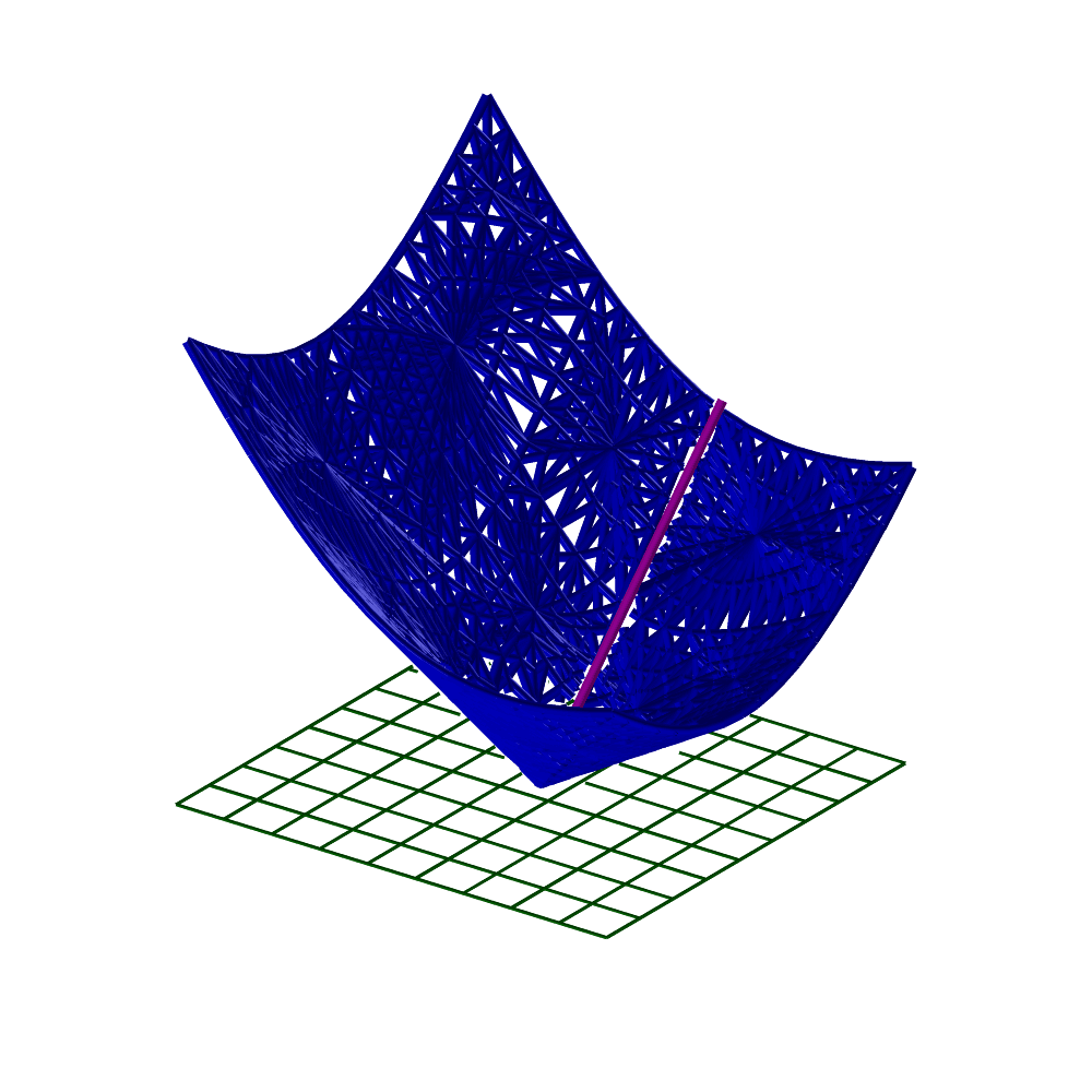
FIGURE: A bisector between two surfaces (left) and a plane and a line (right) computed using MBISECTOR.
MBSPLINE
MultivarType MBSPLINE( ListType Lengths, ListType Orders,
ListType CtlPts, ListType KVLst )
creates a Bspline polynomial/rational multivariate out of the provided control mesh of lengths Lengths and orders Orders in each axis. The sizes of Lengths and Orders define the number of dimensions that the multivariate has. CtlPts is a linear list of control points. All control points must be of type (E1-E9, P1-P9), or regular PointType defining the multivariate's control mesh. The multivariate's point type will be of a space which is the union of the spaces of all points. KVLst is a list of knot sequences of the new Bspline multivariate.
Example:
MV = MBSPLINE( list( 3, 3 ), list( 3, 3 ),
list( ctlpt( E1, 0 ),
ctlpt( E2, 0.25, 1 ),
ctlpt( E3, 0.5, 0.25, 2 ),
ctlpt( E3, 0.5, -1, 3 ),
ctlpt( E3, 0.75, 0.25, 4 ),
ctlpt( E3, 1, -0.5, 5 ),
ctlpt( E3, 1, 0, 6 ),
ctlpt( E3, 1.25, 1, 7 ),
ctlpt( E3, 1.3, 0.25, 8 ) ),
list( list( kv_open ),
list( kv_open ) ) );
constructs a bivariate quadratic multivariate object. See also MPOWER and MBEZIER.
MDERIVE
MultivarType MDERIVE( MultivarType MV, NumericType Dir )
returns a vector field multivariate representing the differentiated multivariate MV, in the given direction. Evaluation of the returned multivariate at a given parameter value will return a vector tangent to TV in Dir at that parameter value.
DMV = MDERIVE( MV, 2 );
computes the partial derivative of the multivariate MV with respect to its second variable. See also CDERIVE, SDERIVE, and TDERIVE.
MDIVIDE
MultivarType MDIVIDE( MultivarType MV, ConstantType Direction,
NumericType Param )
subdivides a multivariate into two at the specified parameter value Param in the specified Direction. MV can be either a B-spline multivariate in which Param must be contained in the parametric domain of the multivariate, or a Bezier multivariate in which Param can be arbitrary, extrapolating if not in the range of zero to one.
It returns a list of the two sub-multivariates. The individual multivariates may be extracted from the list using the NTH command.
Example:
MvDiv = MDIVIDE( Mv2, 3, 0.3 );
Mv2a = nth( MvDiv, 1 ) * tx( -2.2 );
Mv2b = nth( MvDiv, 2 ) * tx( 2.0 );
subdivides Mv2 at the parameter value of 0.3 in the direction 3 and then extracts the two subdivided multivariate. See also CDIVIDE, SDIVIDE, and TDIVIDE.
MDLFILLET
ModelType MDLFILLET( TrivarType TV1, TrivarType TV2,
NumericType Bndry1, NumericType Bndry2,
NumericType RailDist, NumericType R1Orient,
NumericType R2Orient, NumericType TanScale,
NumericType CtlPts, NumericType Tol,
NumericType NumerTol, NumericType FilletingMethod)
Constructs a B-rep model from the boundary surfaces of a (list of) fillet
trivariate(s) that fill the space between the specified boundary surfaces of TV1 and TV2. The fillet meets with the boundary surfaces of TV1 and TV2 with G1 continuity, and it is bounded in between their intersection curve and two rail curves, that are computed as an approximate Euclidean offest of the intersection curve on each of the surfaces. Bndry1 and Bndry2 specify the boundary surfaces of TV1 and TV2 to construct a fillet in between (0,1,2,3,4,5 for UMin, UMax, VMin, VMax, WMin and WMax, respectively, and 6 to take a list of all six boundary surfaces). R1Orient{ and R2Orient specify the orientations of the two rail curves ((+/-)1), or can be set to zero to choose the orientation resulting with the maximal arc length rail curve. TanScale specifies the magnitude of the fillet's tangets that connect it with Srf1 and Srf2.
CtlPts controls the number of control points used to approximate some of the curves computed during the filleting algorithm. Tol and NumerTol specify the tolerances used during the filleting algorithm. FilletingMethod specifies the used filleting method (0 for the ruled volume method and 1 for the volumetric boolean sum method).
Example:
Teapot = load( "vteapot2htr_tvs" );
VBody = nth( Teapot, 1 );
VSpout = nth( Teapot, 3 );
filletMdl = MDLFILLET( VBody, VSpout, 5, 5, 0.3, 1, -1, 0.25, 20,
5e-2, 1e-10, 0 );
See also VMDLFILLET, TVS2FILLET, TVTTFILLET.
MERGEATTR
AnyType MERGEATTR( ListType List, StringType AttrName, NumericType Options )
given a list object List, all elements in the list that contain
AttrName] attribute, and share the same attribute type and value are
merged into one new object. If Options equals 1, a new list object
is returned with the collected elements. If Options equals 2,
similar geometry type (curves or polygons, etc.) are merged into one
object of that type.
Example:
OnlyWithRGB = MERGEATTR( List, "rgb", 1 );
Extracts and merges into a new list that is returned, only elements in
List that have an "rgb" attribute.
See also MERGELIST, MERGEPOLY, MERGEPLLN, MERGETYPE, SPLITLST, FLATTENHIER.
MERGELIST
AnyType MERGELIST( ListType List )
merges a list (of lists recursively) of objects of one single (leaf) type in
List into a single object type (where a linked list of such objet may
result.
Example:
Crvs = MERGELIST( ListOfListOfCrv );
See also MERGEATTR, MERGEPOLY, MERGEPLLN, MERGETYPE, SPLITLST, FLATTENHIER.
MERGEPLLN
PolygonType MERGEPLLN( PolygonType PolyList, NumericType Eps )
or
PolygonType MERGEPLLN( ListType PolyList, NumericType Eps )
merges a set of polylines/polyline objects in PolyList to larger polyline
object. All elements in the PolyList in the second form must be of
PolygonType type. This function merges two polylines if their end point is the
same upto Eps.
Example:
Vrtx1 = vector( -3, -2, -1 );
Vrtx2 = vector( 3, -2, -1 );
Vrtx3 = vector( 3, 2, -1 );
Vrtx4 = vector( -3, 2, -1 );
Polys = list( poly( list( Vrtx1, Vrtx2 ), true ),
poly( list( Vrtx3, Vrtx2 ), true ),
poly( list( Vrtx3, Vrtx4 ), true ),
poly( list( Vrtx1, Vrtx4 ), true ) );
Polys = MERGEPLLN( Polys, 1e-6 );
will merge the four 2-vertices polylines into one polyline prescribing
a square. Note polylines might be reversed in the merging process.
See also MERGEATTR and MERGEPOLY, MERGELIST, MERGETYPE, SPLITLST.
MERGEPOLY
PolygonType MERGEPOLY( ListType PolyList )
merges a set of polygonal objects in the PolyList list to a single polygonal
object. All elements in the ObjectList must be of PolygonType type. This
function performs the same operation as the overloaded ^ operator
would, but may be more convenient to use under some circumstances.
Example:
Vrtx1 = vector( -3, -2, -1 );
Vrtx2 = vector( 3, -2, -1 );
Vrtx3 = vector( 3, 2, -1 );
Vrtx4 = vector( -3, 2, -1 );
Poly1 = poly( list( Vrtx1, Vrtx2, Vrtx3, Vrtx4 ), false );
Vrtx1 = vector( -3, 2, 1 );
Vrtx2 = vector( 3, 2, 1 );
Vrtx3 = vector( 3, -2, 1 );
Vrtx4 = vector( -3, -2, 1 );
Poly2 = poly( list( Vrtx1, Vrtx2, Vrtx3, Vrtx4 ), false );
Vrtx1 = vector( -3, -2, 1 );
Vrtx2 = vector( 3, -2, 1 );
Vrtx3 = vector( 3, -2, -1 );
Vrtx4 = vector( -3, -2, -1 );
Poly3 = poly( list( Vrtx1, Vrtx2, Vrtx3, Vrtx4 ), false );
PolyObj = MERGEPOLY( list( Poly1, Poly2, Poly3 ) );
See figure for an example.
FIGURE:
Individual polygons can be merged into a complete model using MERGEPOLY.
See also INSERTPOLY, SPLITLST, MERGELIST.
MERGETYPE
ListType MERGETYPE( ListType Obj, ConstantType MergeType,
NumericType Tol, NumericType Dir )
Traverses the list object Obj and fetches all objects of type
MergeType from.
MergeType can be one of point_type, vector_type, ctlpt_type,
poly_type, curve_type, surface_type, trimsrf_type, trivar_type, model_type,
multivar_type.
Then, aim to merge the objects along their shared boundaries, if possible, and
when Tol sets the accuracy for deciding if two boundaries are the same and
hence shared.
For types of more than one dimension (i.e. surfaces or trivariates), Dir
sets the direction along which to try and merge.
Example:
M = splitlst( MERGETYPE( M, trivar_type, 1e-5, depth ) );
Aims to merge all trivariates in M along depth. Since MERGETYPE
returns a single trivariate object with a list of trivariate, splitlst is used
to return a list object of objects with a single trivariate in each.
See also MERGEATTR, MERGEPOLY, MERGEPLLN, MERGELIST, SPLITLST.
MEVAL
CtlPtType MEVAL( MultivarType MV, ListType Params )
evaluates the provided multivariate MV at the given Params
values. Params is a list of NumericTypes of length equal to the
dimension of the multivariate that must be contained in the multivariate
parametric domain, if MV is a B-spline multivariate, or all between zero
and one if MV is a Bezier multivariate. The returned control point has the
same type as the control points of MV.
Example:
CPt = MEVAL( MV1, list( 0.1, 0.25, 0.22, 0.7 ) );
evaluates the four-variate MV1 at the parameter values of
(0.1, 0.25, 0.22, 0.7).
See also CEVAL, SEVAL, TEVAL.
MFROM2IMG
CurveType MFROM2IMG( StringType Img1, StringType Img2,
NumericType DoTexture, GeometricType Blob,
NumericType BlobSpread, NumericType BlobColor,
NumericType Resolution, NumericType Negative,
NumericType Intensity, NumericType MinIntensity,
NumericType MergePolys )
Constructs a 3D model of numerous tiny blobs that looks like Img1
from one view direction, like Img2 from another view direction.
DoTexture TRUE adds UV paramterization to the geometry so it can be
used with textures.
If Blob cis a geometric object, it is used as the (tiny) blob element.
Otherwise a cross blob is employed. Blob must be normalized in size to
[0, 1]^3 unit cube. If blob coloring methods are used, it must be a list of
three different geometries to be used for the three different axes.
BlobSpread sets the blobs spreading methods to be used. 0 for random
placement and 1 to 7 for seven different placements along 3D diagonal planes.
Set BlobColor to 0 for no color, 1 for gray levels, and 2 for colored
blobs.
Resolution sets the number of blobs to position in each axes of the
three dimensional cube of blobs.
If Negative TRUE, dark blobs are positioned over light background.
If FALSE, light blobs over dark background is used.
Intensity controls the gray scaling factor.
MinIntensity prescribes the minimal level. if zero, blobs might be
scaled to zero in one diemsion which will make it difficult to manufacture
this model.
Set MinIntensity to TRUE to merge all polygons in the different blobs
into one object.
Example:
resolution = 6;
Blob = sphere( vector( 0, 0, 0 ), 0.35 );
M1 = MFrom2Img( "BenGurion.ppm", "Herzel.ppm",
FALSE, Blob, 0, 0, 25, FALSE, 1.0, 0.01, TRUE )
See figure for an example.
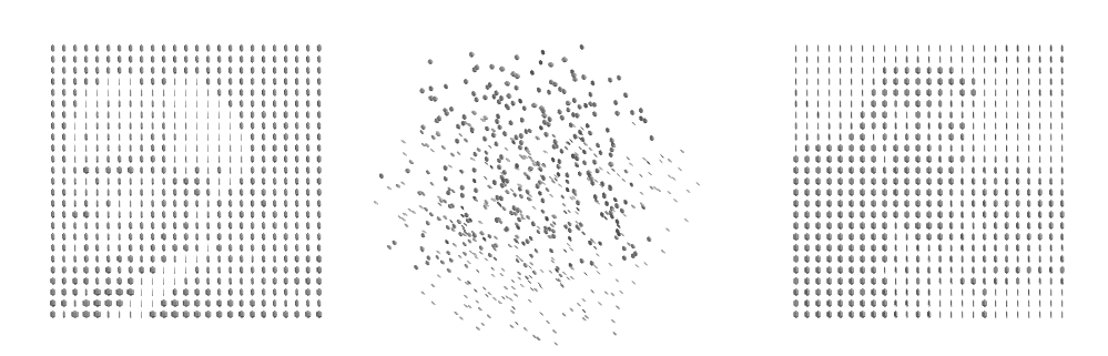
FIGURE:
A 3D model consisting of many small spherical blobs mimics one
image from one view and a different image from an orthogonal view.
Model constructed using the MFROM2IMG command. Left image shows
Ben Gurion, right image shows Herzl and the middle image is a general
view of the 3D model.
See also MFROM3IMG, BFROM2IMG and BFROM3IMG.
MFROM3IMG
CurveType MFROM3IMG( StringType Img1, StringType Img2, StringType Img3,
NumericType DoTexture, GeometricType Blob,
NumericType BlobSpread, NumericType BlobColor,
NumericType Resolution, NumericType Negative,
NumericType Intensity, NumericType MinIntensity,
NumericType MergePolys )
Constructs a 3D model of numerous tiny blobs that looks like Img1
from one view direction, like Img2 from another view direction,
and like Img3 from a third view direction.
DoTexture TRUE adds UV paramterization to the geometry so it can be
used with textures.
If Blob cis a geometric object, it is used as the (tiny) blob element.
Otherwise a cross blob is employed. Blob must be normalized in size to
[0, 1]^3 unit cube. If blob coloring methods are used, it must be a list of
three different geometries to be used for the three different axes.
BlobSpread sets the blobs spreading methods to be used. 0 for random
placement and 1 to 7 for seven different placements along 3D diagonal planes.
Set BlobColor to 0 for no color, 1 for gray levels, and 2 for colored
blobs.
Resolution sets the number of blobs to position in each axes of the
three dimensional cube of blobs.
If Negative TRUE, dark blobs are positioned over light background.
If FALSE, light blobs over dark background is used.
Intensity controls the gray scaling factor.
MinIntensity prescribes the minimal level. if zero, blobs might be
scaled to zero in one diemsion which will make it difficult to manufacture
this model.
Set MinIntensity to TRUE to merge all polygons in the different blobs
into one object.
Example:
M2 = MFrom3Img( "BenGurion.ppm", "Herzel.ppm", "Rabin.ppm",
FALSE, FALSE, 1, 1, 40, FALSE, 1.0, 0.01, 1 );
See also MFROM2IMG, BFROM2IMG and BFROM3IMG.
MFROMMESH
MultivarType MFROMMESH( MultivarType MV, MumericType Dir, NumericType Index )
extracts a multivariate out of a multivariate, MV, as the Index's
plane of the control mesh of MV in direction Dir.
Example:
cmesh( s, row, 2 ) ==
coerce( MFROMMESH( coerce( s, multivar_type ), 1, 2 ), curve_type );
coerces surface s to a multivariate, extracts a one-dimensional-less
multivariate (a curve) from the second direction (first direction is
direction zero), at index 2 and compares the result for equality to
the curve extracted using cmesh from s.
MFROMMV
MultivarType MFROMMV( MultivarType MV, NumericType Dir, NumericType Param )
extracts a multivariate of one lower dimension from multivariate MV by
extracting an iso-variate of MV in direction Dir at parameter
value Param.
Example:
MVFirst = MFROMMV( MV, 0, FirstParam );
extracts a multivariate for one less dimension than MV as the
constant first parameter of MV at parameter value FirstParam.
See also STRIVAR, CSURFACE.
MICROBREPSTRCT
ListType MICROBREPSTRCT( SurfaceType Srf | TrimSrfType TrimSrf |
ModelType Mdl | VModelType VMdl | PolygonType Poly,
ListType Tiles, TrivarType TileCage,
ListType TileParam )
Construct microtiles in a B-rep macro object. The first parameter
represents the boundary of the B-rep macro object, which can be one
of the following types: a spline surface, a trim surface, a Model, a
V-Model, or a polygonal model. Tiles is a list of microtiles
constructed using the MICROSTRCT command and the trivariate
TileCage that typically will conatins the input B-rep object,
serving as its cage. Microtiles must be constructed by the regular
tiling option in MICROSTRCT. Each tile consists of trivariates,
surfaces, or curves. Among the microtiles, only the tiles that are
fully inside the B-rep macro object are kept and other tiles, that
are either fully outside the macro object or intersecting with the
boundary of the macro object, are purged. For each inside tile,
anchors are identified from the boundary elements of the tiles and
bridged to the closest location on the macro B-reps, using bridging
tiles. Surface anchors are used in trivariate and surface tiles and
point anchors are used in curve tiles.
TileParam is a list of parameters used in constructing
bridging tiles, which connect anchors to the macro B-reps.
TileParam is specified as list(NrmScale, NrmBlendingRatio,
OutletSrfScale), as folows:
1. NrmScale is a scale parameter that controls the length of
start and end direction vectorss of the sweeping axes of
bridging tiles. The length of directions is equal to the
distance between start and end points multiplied by NrmScale.
2. NrmBlendingRatio is a scale parameter that controls the
direction of sweeping axis curves of the bridging tiles. If 0,
then the starting direction of an axis curve derives from the
derivative of the trivariate adjacent to the anchor. If 1, the
direction derives from the surface normal of the anchor.
Only used in trivariate tiles.
3. OutSrfScale is a scale parameter to scale the surfaces of
bridging tiles with respect to inlet anchors. Only used in
trivariate and surface tiles.
The output is a list of two lists, where the first list is a list
of tiles that are fully inside the macro object (originated from
input Tiles) and the second list is a list of bridging tiles.
Example:
MacroObj = load("Model.stl"); # A Brep polygonal model
Tiles = MicroStrct( TV, 1, list( Tile1, 0, 0, True, list( 5,5,5 ),
True, 0, 1.0, 4, False, False ) );
TilesBRep = MicroBrepStrct( MacroObj, Tiles, TV, list( 0.3, 0, 0.8 ) );
loads the polygonal macro model "MacroObj", and construct
microtiles filling a deformation map TV with the regular tiling, and
select the tiles inside MacroObj and connect them to the boundary of
MacroObj with bridging tiles. (Assume Tile1 is a trivariate tile, the
start direction of each sweeping axis curve derives from the
derivative of adjacent tile trivariate and the length of the
direction is the distance between the start and end points multiplied
by 0.3. The outlet surfaces of bridging tiles are scaled from the
inlet anchor surfaces by 0.8.)
See also: MICROSTRCT, MICROTILE, MICROVMSTRCT
MICROSLICE
PolyType MICROSLICE( NumericType NumLevels,
VectorType ZRange,
TrivarType DeformTrivariate,
ListType Params,
ListType LevelParams,
ListType Tolerances )
Computes planar slices of a computed (recursive) microstructure. The
generation of the microstructure is handled by the parameters
DeformTrivariate, Params, and LevelParams.
DeformTrivariate is as in the MICROSTRCT command's deformation
function that is used to deform the resulting microstructure. While
this function constructs regular microstructures in the same way
MICROSTRCT does, it does so recursively (hierarchically) and a lazy
way, due to memory constraints, and as needed per planaer slice.
That is, after operating as MICROSTRCT, and creating a number of
microstructure cells, each cell is (recursively) used as the new
DeformTrivariate of a new regular microstruture, recursively.
Params are again the same as in MICROSTRCT, and are used as
the default value for microstructure parameters. LevelParams
allow setting specific Params parameters for each recursive
level of the microstructuring process. Each element in LevelParams
is a tuple with the level number and the specific Params paramters
for that level.
NumLevels determines the number of recursive microstructure
levels. ZRange is a vector with the first (ZRange[0]), last
(ZRange[2]), and delta (ZRange[1]), z coordinate values at which the
microstruture will be sliced. At each slicing level (z = values) the
outline of the microstructure will be determined using the
intersection of the boundary surfaces of the microstructure's
hierarchy and the z = value plane.
Finally, the tolerances used by the solver in this case are determined
by the last Tolerances parameter, ordered as (numeric,
subdivision, tracing, and angular deviation) toleraces. The outline
will be returned as a polygonal object (set set of planar polylines).
Note that this piecewise linear output will be pruned to the
elimination of adjacent edges with small angles' deviations in the
parametric domain.
Example:
S = MICROSLICE( 2, vector( 0.0001, 1.0002, 0.249 ), UnitTV,
list( Cn, True, vector( 1, 2, 1 ),
true, 0.5, false, 1.0, 3, false ),
list( 0, list( Cn, True, vector( 1, 2, 1 ),
true, 0.5, false, 1.0, 3, false ),
1, list( Boxes, True, vector( 2, 2, 2 ),
true, 0.5, false, 1.0, 3, false ) ),
list( 0.001, 0.0005, 1e-10, 0.02 ) );
constructing slices between (almost) zero and (almost) one in steps of
(almost) 1/4, in a two-levels hierarchy.
See also VMSLICE
MICROSTRCT
AnyType MICROSTRCT( TrivarType DeformTrivariate,
NumericType TilingType,
ListType Params )
Computes a microstructure by tiling the domain and then deforming the
same using DeformTrivariate.
The parameter TilingType determines whether to apply regular
tiling (TilingType = 1), functional tiling (TilingType = 2
NOT supported via the IRIT scripting langauge - only in C code,
random grid tiling (TilingType = 3), implicit and random tiling
with bifurcation (TilingType = 4) or regular tiling with
bifurcation (TilingType = 5). Other parameters for tiling are
supplied via Params.
For regular tiling (TilingType = 1), Params includes the
following parameters:
1 The first parameter is the tile which is repeated within the domain
of DeformTrivariate. The tile may be a polyline, a curve,
a surface, a trimmed surface, a polygon, or a trivariate, or a mix
of these. The tile must fit the unit cube, [0, 1]^3.
If, however, the tile is a list object and the 1st parameter is a
number n, as list( n, T1, ..., Tn ) with n={ 2,3 } additional objects
in the list, these tiles are used in order, in the W direction of the
DeformTrivariate. if n = 2, exactly two tiles are to be placed
in the w direction. If n = 3, three or more tiles are to be placed in
the w direction with first tile in the list is first in w, middle tile
is interior to the microstructure and last tile in the list is a
terminating tile in w.
Further, if the tile is a list object with six sub-objects and the
first, second, fourth and/or fifth parameters is a string, the tile
is considered parameteric in the form defined in MICROTILE,
TileType 1. Here, the first, second, fourth, and/or fifth parameters
can be strings, in which case they prescribe an arbitrary function
in UVW (the domain of DeformTrivariate) and/or xyz (Euclidean
locations). The locally evaluated value of the function (i.e. outer
radius) serves to prescribed the local geometry of the tile.
2 Shelling and/or capping may be applied to the boundary of the
microstructure, as specified by bits in ShellBits, as follows
(lsb to msb): CapUMin, CapUMax, CapVMin, CapVMax, CapWMin, CapWMax,
ShellUMin, ShellUMax, ShellVMin, ShellVMax, ShellWMin, ShellWMax,
where Cap means close any opening in the tile on that boundary and
shell means close the entire face as a complete shell.
If, however, This capping info equals -1, automatic capping to
tiles that are either SURFACE_TYPE or MODEL_TYPE will be aimed.
3 If shelling is specified by one or more bits of the 2nd parameters
then the thickness of the wall (in parameter space's tile unit cube)
is set here.
4 This parameter specifies the interpretation of the repetition rates
of tiles in three different directions within each Bezier domain
of DeformTrivariate. A value of TRUE means number of tiles'
repetition and a value of FALSE means displacements in UVW doamin,
in parameter space, and can be fractional.
5 This parameter, which is a list of size three of either integers/
reals or list-of-integers/reals specifies either repetition rates or
displacements of tiles within the domain, as directed by the previous
parameter. In any direction, integers/reals or the
list-of-integers/reals, Vi, specify the tiles repetition counts
(dispacements) for different Bezier patches (i,e, for every knot
interval), as (V1, V2, ..., Vn), for n different knot intervals.
If only an integer/real is specified, it is used for all knot
intervals in that direction.
Note that if a direction has > n intervals, each Vi value will
be affecting a larger zone than a single knot interval.
6 Specifies whether the trim-curves of trimmed surfaces in the tiles
should be approximated first as piecewise linear curves.
7 Specifies the scaling in the w-direction in case of trivariate tiles
with G0-discontinuity. In the case of such tiles, the repetition
factor gets multiplied by the number of G0-discontinuities in u and
v directions, at each level in w-direction. A set of refinement
matrices are returned for each discontinuity, as an
"UKnotRefineMatrix" and "VKnotRefineMatrix" attributes.
8 Specifies the maximum edge-length in case of polygonal tiles.
Polygons with edge-length(s) larger that this specification, are
subdivided (to ensure desired approxiamtion after deformation).
9 Specifies if low order approximation is to be applited to the output,
with 0, 3 or 4 indicating non, quadratic or cubic approximation.
Applies for curves, surfaces, and trivariates.
10 Indicates whether the tiling specification is global, i.e., for the
entire domain of the deformation function. A side effect of this (if
TRUE) is that tiles are likely to cross knot lines and be subdivided
(surfaces into trimmed surfaces, etc.).
11 Indicates whether a free-form deformation approximtion is to be
applied instead of precise functional composition of tiles.
Notes on the regular tiling:
Created tiles in the microstructure will have the following attributes:
"MSTileID" which will hold unique integer ID (starting from one).
"BzrIndex" as a string attribute that holds the Bezier domain indices
in the global (possibly B-spline) input deformation mapping, like
"0,0,0" for the first domain (or the only domain if global B-spline
deformation function).
"MSIndex" as a string attribute that holds the tile indices in the local
(Bezier polynomial) deformation function, starting from zero, like
"0,0,0", and,
"DmnBBox" that will hold the domain of this local polynomial deformation
function in the global (possibly B-spline) input deformation function.
The domain of an individual tile in the global deformation function can
be deduced from the above, as the "MSIndex" is uniformly dividing
"DmnBBox".
If the tiles are trivariates and Cap* bits are set, two additional types
of attributes are going to be set for trivariates that are on the
boundary of the deformation mapping. An integer attribute
"MSDfrmTVBndryU", and/or "MSDfrmTVBndryV", and/or "MSDfrmTVBndryW", if
this trivariate is on the U/V/W boundary and the integer value will be
0 to 5, denoting the UMin, UMax, VMin ... WMax of the deformation function.
Further, if attribute(s) "MSDfrmTVBndryU", or "MSDfrmTVBndryV", or
"MSDfrmTVBndryW" is/are set, a second corresponding set of attributes
(that U/V/W correspond to the "MSDfrmTVBndryU/V/W" attributes) of
"MSLclTVBndryU", or "MSLclTVBndryV", or "MSLclTVBndryW" will be defined
in local trivariate with integer value of 0 to 5, denoting the UMin,
UMax, VMin ... WMax boundary of this local trivariate that is on the
boundary of the deformation TV.
Finally, dim and light RGB colors will be set for these min/max U/V/W
boundaries, respectively (i.e. R for U, G for V, and B for W) of the,
deformation function on each such boundary trivariates.
Example for regular tiling:
M = MICROSTRCT( DefMap, 1,
list( Tile, 0, 0, True, list( 2, 2, 2, 2 ),
True, 0, 1.0, 0, False, False ) );
See figure for an example.
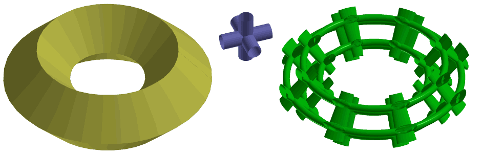
FIGURE:
A microstructure constructed inside a square-cross-section torus (left)
and a 3D cross-like tile (middle). The torus on the left is a
trivariate and the tile is a MODEL - a Boolean operation between.
three surfaces. The microstructure result is shown on the right.
For random tiling in a uniform grid (TilingType = 3), each cell
in the grid is assigned a scalar (randomized) trivariate, and the tile's
geometry is the zero set of the trivariate, and presents the necessary
continuity. Params includes seven parameters:
1 Number of the tiles at each parametric direction (a vector of three
numbers).
2 The orders of trivariate at each direction (a vector of three numbers).
3 The number of the control coefficients of the trivariate at each
direction (vector of three).
4 The minimal trivariate coefficient value.
5 The maximal trivariate coefficient value.
6 A Boolean value (true of false) that states if the connectivity
between the tiles should be C^1 continuous (true) or C^0 (false).
7 A boolean value that states if to use a graph consisting of two
spanning trees that determines the connectivity between the tiles,
and ensures inter- and intra-connectivity of the tiles.
Example for random tiling of a grid of eight tiles at each direction,
and using trivariate of order three (quadratic) at each direction and
having six control coefficients at each direction, whose values are
randomly set from the range [-1,1]. The tiles are C^1 continuous,
and connectivity graph is used:
MRandom = MICROSTRCT( DefMap, 3,
list( vector( 8, 8, 8 ), vector( 3, 3, 3 ),
vector( 6, 6, 6 ), -1, 1, true, true ) );
For implicit bifurcation tiling (TilingType = 4), the parametric
space is adaptively subdivided into boxes, such that the length of
the edges of the box in the Euclidean space doesn't exceed a given
threshold. Each tile in the non uniform adaptive grid is assigned a
scalar trivariate, and the tile geometry is the zero set of the
trivariate. Bifurcation tiles are automatically generated to connect
tiles with different neighboring topologies. Params includes
four parameters:
1 The orders of the trivariate at each direction (vector of three) for
each tile.
2 The number of the control coefficents of the trivariate at each
direction (vector of three). (For bifurcation tiles, there will be
more).
3 The subdivision threshold.
4 A number between 0 and 1, which controls the randomness of the tiles.
0 means no randomness (the basic tile is a tubical cross) and 1 is
fully random (except at places where connectivity should be ensured).
Example for random tiling with implicit bifurcation, using trivariate
of order 3 and 8 control points at each direction for the basic
tile. The subdivision threshold in the Euclidean space is 0.7, and
the randomness factor is 0.1:
MRandom = MICROSTRCT( DefMap, 4,
list( vector( 3, 3, 3 ), vector( 8, 8, 8 ),
0.7, 0.1 ) );
For regular tiling bifurcation tiling (TilingType = 5), the basic
tile and the bifurcation tiles should be provided. The parametric
space is adaptively subdivided into boxes (restricted to the provided
bifurcation topologies). The supported bifurcation topologies are:
1x1, 1x2, 1x4, 2x2. and the bifurcation is restricted to be along one
direction only. Params includes four parameters:
1 The subdivision direction - 0 for u, 1 for v, and 2 for w.
2 The subdivision threshold.
3 Approximation lower order. 0 to disable, 3 or 4 for tri-quadratic
or tri-cubic lower order approximations of the resulting geometry.
4 A list of tile objects, organized in the following order:
(basic tile, 1 to 2 bifurcation tile, 1 to 4 bifurcation tile,
2 to 2 bifurcation tile). Except for the basic tile, the other tiles
can be nil() if that bifurcation topology will not be encountered.
The tiles can be of any (combination of any) geometry type.
5 Indicates whether a free-form deformation approximtion is to be
applied instead of precise functional composition of tiles.
Notes on the design of the bifurcation tiles:
The orientation of the bifurcation tiles should match the
bifurcation direction provided in the first parameter in the param
list.
The bifurcation tiles have branch in and branch out
boundaries. These boundaries should be designed such that each
branch out boundary should match the branch in boundary exactly
after scaling to the same size and aspect ratio. For example,
examining a 1x2 bifurcation surface tile, which has a circular
boundary branch in and branch out curves. The branch out curves
should be an ellipse which is the branch in circle scaled by (0.5,
1) in the (u,v) directions, respectfully. The position of the
boundary also should match, such that it will have the same position
relative to the containing box in the parametric space.
In case of 1X2 and 1X4 bifurcation tiles, the split of the geometry
(towards the branch out boundaries) should be along the next
parametric direction after the bifurcation direction. For example,
for 1X2 bifurcation tile, if the bifurcation direction is along the
w direction, then the two branch out boundaries should be along the
u direction, such that the boundary of the two branch outs should
have the same v and w values, and only translated along the u
direction.
Example for random tiling with regular bifurcation, allowing
bifurcation in the w direction with subdivision threshold in the
Euclidean space of 0.7, and no lower order approximations:
MRandom = MICROSTRCT( DefMap, 5,
list( 2, 0.7, 0,
list( Tile11p, Tile12p, Tile14p, Tile22p ),
true ) );
See also MICROBREPSTRCT, MICROTILE and MICROVMSTRCT.
MICROTILE
PolyType MICROTILE( NumericType TileType, ListType Params )
generates a tile, compatible with the tiles needed by the MICROSTRUCT command
interface, in [0, 1]^3. TileType controls the type of tyle generated
while Params controls the parameteris, as follows:
If TileType == 1, a 3D Cross tile is created with faces in all six
directions (+/-U, +/-V, +/-W). Params includes a list of six faces
parameters, corresponding to the expected UMin, UMax, VMin, VMax,
WMin, WMax faces, in this order and a last 7th parameter that if TRUE,
requests to also synthesize the negative (free) space in the tile. The
negative space is supported only if the tile is solid (inner radius is
zero) and no boundary. Each face parameters is, in itself, a list of
eight parameters as follows:
1 Outer radius of branch on the face.
2 Inner radius of branch on the face. Can be Zero to make solid.
3 A Yscale factor of the face cross section, assuming in the XY
plane, creating an elliptic instead of circular face cross section.
4 Boolean flag - TRUE for a circular cross section, FALSE for
rectangular.
5 A bounday rounding shape control. A number between zero and one
to affect how the geometry is rounded going into the face.
6 A list of four numbers as expected skin thickness at these four
corners of that face. If all four values are zero, or this list
is empty (nil()), no skin geometry is generated.
7 A list of three center location points, in, [0, 0.5]^2, to shift
the center joints on the respective face, or nil() to disable.
A very large negative coordinate value, <-1e6, will force the
branch to be straight (vertical in Z, for example).
8 A list of three numeric parameters, requesting a helical arm with
(NumberLoops, MajorRadius. MinorRadius) as the parameters of the
created helical arm.
If all three parameters are zero, or the list is nil(), then this
option is disabled.
Notes:
Tile will consist of complete tensor product trivariates only.
A tile can be either completely hollowed or completely solid
(that is, all Inner Radii are zero or all are positive, but
not necessarily the same).
A tile can have a full face skin in one face or two (opposite)
faces only.
Example:
FacePrm = list( 0.125, 0.1, 1.0, true, 0.5, nil(), nil() ):
Tile = MICROTILE( 1,
list( FacePrm, FacePrm, FacePrm,
FacePrm, FacePrm, FacePrm, FALSE ) );
creates a hollowed tile with rounded cross sections and no skin, in
all six faces and no negative space.
If TileType == 2, a bifurcation tile is created with one main
branch in ZMin and two branches in ZMax. Params starts with
lists of parameters of three faces, corresponding to the expected ZMin,
ZMax1, ZMax2 faces, in this order. Each list of face parameters is,
in itself, the same as the face parameters of TileType of type 1,
up to the last parameter that does not exist.
The three last parameters, control, in order, the gap size between the
branching out faces (between ZMax1 and ZMax2), the rounded shape of the
saddle between them, and whether to return tensor product trivariates
(TRUE) or tensor product surfaces (FALSE).
Example:
ZMinFacePrm = list( 0.2, 0.0, 1.0, false, 0.0, nil(), nil() );
ZMaxFacePrm = list( 0.125, 0.1, 1.0, true, 0.5, nil(), nil() );
Tile = MICROTILE( 2, list( ZMinFacePrm, ZMaxFacePrm, ZMaxFacePrm,
0.25, 0.05, true ) );
creates a hollowed bifurcation tile with rectangle cross sections,
as of trivariates.
If TileType == 3, a shell lattice tile is created using a
semi regular tesselation. Params is a list of three parameters
as
(SemiRegType, TileGeomType, TileSize),
where SemiRegDualType is one of 848, 1246, 4346, 6363, 12312,
33336, 44333, 43433, TileGeomType can be one of:
0 univariate planar curves tiles.
1 bivariate planar surfaces tiles.
2 trivariate extruded into 3D tiles.
TileSize sets a scaling factor on the tile.
Example:
D12312 = microtile( 3, list( 12312, 2, 0.15 ) );
If TileType == 4, a shell lattice tile is created using dual
semi regular tesselation. Params is a list of five parameters
as
(SemiRegDualType, TileGeomType, TileSize, Indent, CrvAmt,
RectangularTiling, NormalizeRectangle),
where SemiRegDualType is one of 848, 1246, 4346, 6363, 12312,
33336, 44333, 43433, TileGeomType can be one of:
0 univariate closed planar curves tiles.
1 univariate open planar curves tiles.
2 bivariate planar surfaces tiles.
3 trivariate extruded into 3D tiles.
4
5
TileSize sets a scaling factor on the tile, Indent
([0, 1] prescribes the fraction of a tile edge that is used in
the dual synthesized geometry, CrvAmt controls the curvature
of the constructed geometry.
RectangularTiling and NormalizeRectangle are optional.
The parameter NormalizeRectangle is used only if
RectangularTiling is TRUE.
RectangularTiling is TRUE to create (if possible) a rectangular
repeatable macro tile (FALSE by default).
NormalizeRectangle is TRUE to normalizes extracted rectangle
to unit square / cube.
Example:
D12312 = microtile( 4, list( 12312, 2, 0.15, 0.8, 0.5 ) );
If TileType == 5, a spring flexible tile where Params
includes four items, as
( SpringOrder, Point( SpringWidth, SpringTrans, SpringScale ),
list( UMinArmWidth, UMaxArmWidth, VMinArmWidth, VMaxArmWidth ),
ArmsHeight )
where SpringOrder is the spline order of the spring and can be
2 (linear) or 3 (quadratic), SpringWidth, SpringTrans],
SpringScale controls the width (typically < 0.3), extent
([-0.5, 0] for linear springs, [-0.5, 0.9] for quadratic springs),
and size ([0.1 to 2]) of the spring. The size *ArmWidth
control the XY crosses ([0.01, 1.9]), and ArmsHeight the height
of these XY crosses.
Example:
Tile = microtile( 5, list( 3, point( 0.2, 0.4, 1.2 ),
list( 0.4, 0.4, 0.4, 0.4 ), 0.15 ) );
If TileType == 6, a unit tile is created with diagonal edges.
That is, no edges are horizontal in the tile, a tile that hence can
be used toward 3D printing without support. Params contains
five values:
(CentralJointSize, CornerSizesList, CornerVertScale,
SmoothingFactor, SkinInfo)},
where CentralJointSize is the size of the central cuboid
elements.
CornerSizesList is a list of edge sizes, The list can have 1,
3, 8 or 10 numbers. If 1 or 8 numbers, 8 diagonal edges are created
from the center of the tile to the 8 corners of the tile with
homogoneous thickness (if 1) or different thicknesses (if 8).
If 3 or 10 numbers are specified, the two additional numbers
(above the 1 or 8) signal a need to also add a central vertical up
and/or central vertical down rods. A thickness of zero disables that
rod. If negative, the rod is twsited 45 degrees to be axis parallel.
In addition, CornerVertScale can control the vertical scale of
the corner's boxes, with zero to completely disable the creation of
corner boxes.
Then, SmoothinFactor controls the rounded of the diagonal
edges, if any, or zero to disable (have linear edges).
Finally, Skin holds a pair of numeric values to control
an option of a skin in Y/ZMin and/or Y/ZMax. If either is positive,
a frame is cconstructed and if either is negative, a full skin is
created. Zero to disable Skin/Frame.
Example:
LinDiagTile = microtile( 6, list( 0.15, list( 0.1 ),
1.0, 0.0, list( 0, 1 ) ) );
If TileType == 7, an Auxetic parametric tile is cleated.
Params includes eight items, with the first six are lists
controlling the (XMin, XMax, YMin, YMax, ZMin, ZMax) different
faces of the tile. This face list parameters are
(HasOutJoint, InnerJointDiameter, { PossionRatio })
where HasOutJoint can be 0, 1, or 2 to control the creation of
a joint to the neighboring tile. If 0, no joint to a neighboring
tile is created, for 1, a rigid joint is created, and for 2, a
flexible joint. Flexible joints can be created in XY directions
only. InnerJointDiameter is a positive parameter, setting
the diameter of this faces' bars, and PossionRatio sets the
desired Possion ratio of this specific faces (in ~[-1, 1] range but
also depends on the thicknesses of the bars).
The last two items in the parameter list controls:
CircularBars the shapes of the bars that can be either
circular or rectangle, and FlexClipRatio that (in [0.0, 0.5}
range) sets the range of flexibility that is desired in the
horizonal bars of the tile, at its two ends.
Example:
Wdt = 0.15;
AuxTile = microtile( 7, list( list( 1, Wdt, 0.2 ),
list( 1, Wdt, 0.2 ),
list( 2, Wdt, -0.2 ),
list( 2, Wdt, -0.2 ),
list( 1, Wdt ),
list( 0, Wdt ),
true, 0.15 ) );
creates tile AuxTile with connecting joints toward all neighbors but
ZMax, with a Possion's value of 0.2 in X and -0,2 in Y, with circular
bars of width Wdt, and flexible ratios in the bars of 0.15.
If TileType == 8, a bistable tile is created, meaning a tile
that on impact, can switch state. Can be a 2D planar tile with some
thickness or a full 3D tile.
For a 3D tile, Params includes six items as
(FrameSize, WeightRodsThickness, WeightRodsSpring, WeightRodsAngle,
ClipFlexcRatio, CntrWgtSizes)
FrameSize controls the thickness of the outer rectangle frame
in the [0.0, 0.25] range. WeightRodsThickness
controls the thicknesses of the rods from the frame to the weight, in
the [0.0, FrameSize] range. WeightRodsSpring is zero for
straight joint, and positive for a springy joint (larger value,
larger spring). WeightRodsAngle sets the
angle, in degrees, to position the weights' rods, in the [-45, 45]
range. The large this angle, the larger the neede impact to change
the state. FlexClipRatio controls how much of the weight's
rods are flexible and what portion is rigid, in the [0.0, 0.5] range.
Finally, CenterWeightSizes holds the dimensions of the central
weight in X, Y, Z.
For a 2D tile, Params includes seven items as
(FrameSize, FrameGap, WeightRodsThickness, WeightRodsSpring,
WeightRodsAngle, ClipFlexcRatio, CntrWgtSizes)
where the additional 2nd parameter FrameGap adds optional
hotizontal gap in the frame, on the left and right sides, if
positive, that FrameGap amount.
Example:
BistableTile3D = microtile( 8, list( 0.15, 0.0, 0.02, 0.0, -5, 0.0,
list( 0.2, 0.2, 0.5 ) );
creates a 2D bistable tile.
If TileType == 9, a 4 sided texture rag tile which is a hollowed
cube with one face removed, with texture maps (texture0.png to
texture4.png) on the five remaining faces.
The options get three parameters: (WallThickness, DiagEdge, RetSrfObj)
where (WallThickness defines the wall thickness, DiagEdge
selects between diagonal and horizontal front edges and
RetSrfObj selects if the returned tile is a surface object or a
list object with surface objects in it.
Example:
WallWidth = 0.1;
RagTile1 = microtile( 9, list( WallWidth, false, true ) );
If TileType == 10, a skew/shear tile is created. The options
gets six number values:
( BaseHeight, RodWidth, RodSpace, XTwistShift, MidRodScl, ElasticFrac )
where BaseHeight controls the height of the bottom and top
bases, RodWidth sets the width of the diagonal rods and
RodSpace prescribes the distances between parallel rods.
XTwistShift controls the diagonal X shift amount, per rod, and
MidRodScl allows the scale of the thickness of the rods, in the
middle. Finally, ElasticFrac sets the relative regions in the ends
of the rod that are defined as flexible material.
BaseHeight, RodWidth, and ElasticFrac are in the
[0.0, 0.5] range and RodSpace and MidRodScl in [0.0, 1.0].
Then, XTwistShift can be in [-1.0, 1.0].
Example:
SkewTile = microtile( 10, list( 0.1, 0.1, 0.2, 0.2, 0.5, 0.25 ) );
If TileType == 11, a bending tile is created, in either X or XY.
The options gets four number values:
( ( FlexHeight, FlexWidth ), RigidLength, BendXY, Merged )
where FlexWidthHeight is a list of two numeric vlaues that sets
the dimensions of the central zone of the flexible width (in X) and
height (in Y), in (0, 1) ranges, and RigidLength sets the length
of the left/right rigid zone, in (0, 1) range. Then, BendXY is
TRUE for a tile that bends in both X and Y, FALSE for only X, and
finally, Merged is TRUE to return one geometric object or FALSE
to return two parts of the rigid parts and the flexible one.
Example:
BendTile = microtile( 11, list( list( 0.9, 0.1 ), 0.2, true, false ) );
If TileType == 12, a collapsing bistable tile is created, in either
X or XY. The options gets five number values:
( FrameThickness, JointsSize, SideJointLevel, FlexClipRatio,
HelicalArms )
where FrameThickness controls the thickness of the created
geometry, in (0, 1) range, and JointsSize sets the
length of the left/right/top/bottom joints to neighboring tiles,
again in (0, 1) range. SideJointLevel allows control on the Y level
of the left/right joints. FlexClipRatio prescribes the ratio of
the flexible materials in the flexing arms in (0, 0.5) range.
Finally, HelicalArms can be nil() for regular arms or be a list
of three parameters to control the (NumLoops, MnrRad, MjrRad) of the
helical arms.
Example:
CollapsingTile = microtile( 12, list( 0.15, 0.25, 0.5, 0.25, nil() ) );
If TileType == 13, a collapsing bistable tile in both X and Y is
created. The options gets three numeric values:
( FrameThickness, JointsSize, FlexClipRatio )
where FrameThickness controls the thickness of the created
geometry, in (0, 1) range, and JointsSize sets the
length of the left/right/top/bottom joints to neighboring tiles,
again in (0, 1) range. FlexClipRatio prescribes the ratio of
the flexible materials in the flexing arms.
Example:
CollapsingXYTile = microtile( 13, list( 0.15, 0.25, 0.25 ) );
See also CRVNET2TILE, MICROSTRCT, MICROVMSTRCT and MICROBREPSTRCT.
MICROVMSTRCT
ListType MICROVMSTRCT( NumericType Oper, ListType Params )
constructs micorstructures in a VModel that undergos a sequence of
volumetric Boolean operations, tiling micro-elements inside trimmed
trivariates (VCells). Oper can be:
1 Intializes the process, before volumetric Boolean operations take
place. Here, Param has no effect and can be nil().
2 Creates the microstructure and return it as a list of micro-elements.
Here, Params is list( VModel, NormalScale, NormalBlendingRatio,
SaddleRatio, BoundryMarginRatio,
CheckingJacobian );
See below for the meaning of these parameters.
The parameters in Params, if Oper is 2, are:
VModel:
the resulting model of the volumetric Booleans
NormalScale:
This scale parameter controls the shape of sweeping axis curve in a
bridging tile. The length of the start and end directions of the
sweeping axis curve is determined as the distance between the start
and end points of the curve multiplied by NormalScale.
NormalBlendingRatio:
This parameter determines the direction of deviation of a bridging
tile with respect to its anchoring face. If 0, the direction of a
bridging tile comes from the derivative of the trivariate adjacent
to the inlet anchoring face. If 1, the directions come from the
surface normal of the anchoring faces. Otherwise, the two directions
are blended with NormalBlendingRatio.
SaddleRatio:
This parameter determines the size of saddle in each base trivariate
in a bifurcation tile. It determines the size of top surface of the
base trivariate
BoundryMarginRatio:
If not 0, then additional margin is allowed in the tile membership
test. Larger value makes more inside tiles be classified as
intersecting and be purged away.
CheckingJacobian:
If TRUE, the bridging tiles are constructed to be positive Jacobian
as much as possible. In this case, some parts of the existing tiles
might be further eliminated with the new anchoring faces detected.
Each trivariate/primitive participating in the Booleans must contain
the following attribute information, before it is employed in the
Booleans:
attrib( Prim, "MVMSInfo",
list( Tile,
TileRepeatsList( { XList, X }, { YList, Y }, { ZList, Z } ),
PrimPriority );
where Tile is the tiles to use for this primitive (different
primitives can use different tiles), TileRepeatsList constains
lists of repetition in U, V and W (as in MICROSTRCT) either as a
single number of how many tiles per knot interval, or as a list of
number for tiles per specific knot interval. Finally,
PrimPriority sets a numeric priority to control which primitive
trivariate is more important when have VCells of multiple trivariates
(e.g. Union), and hence its full sets of microstructure will be
employed. Smaller PrimPriority value means higher priority.
Returned tiles are color-coded as follows:
If CheckJacobian is FALSE, then each trivariate is colored
based on its membership with respect to the macro shape Model:
Green - the trivariate originates from an "inside" tile.
Yellow - the trivariate originates from a "to-be-bridged" tile,
which is to be connected using bridging tiles.
Red - the trivariate originates from a "bridging" tile.
If CheckJacobian is TRUE, then each trivariate is colored
based on its margin allowance for positive Jacobian:
Blue - the trivariate is positive Jacobian as it is.
Green - the trivariate is positive Jacobian when the 0.5%
of the parametric domain is clipped in the trivariate
Cyan - positive Jacobian with 1% margin clipping
Red - positive Jacobian with 1.5% margin clipping
Magenta - positive Jacobian with 2.5% margin clipping
Brown - positive Jacobian with 5% margin clipping
Lightgrey - fail to ensure positive Jacobian even with 5% margin
clipping
A full example:
Iritstate( "PrimType", 4 );
CylA = cylin( vector( -0.5, 0, 0), vector( 1, 0, 0 ), 0.25, 3 );
CylB = coerce( CylA, vmodel_type ) * ry( 90 ) * sc( 1.1 );
FacePrm = list( 0.125, 0.0, 1.0, true, 0.2, nil() );
Tile = microtile( 1, list( FacePrm, FacePrm, FacePrm,
FacePrm, FacePrm, FacePrm ) );
attrib( CylA, "MVMSInfo", list( Tile, list( 4, 4, 8 ), 1.0 ) );
attrib( CylB, "MVMSInfo", list( Tile, list( 4, 4, 8 ), 2.0 ) );
MICROVMSTRCT( 1, nil() );
MacroV = CylA + CylB;
MS = MICROVMSTRCT( 2, list( MacroV, 0.3, 0.5, 0.1, 0, 0 ) );
Computes a microstructure for a union of two cylinder, where CylA has
higher priority.
See figure for this example.

FIGURE:
A microstructure constructed inside a VModel that is the union of
two cylinders, using the MICROVMSTRCT command. The regular tiles
are shown in green, the bridging tiles (inbetween primitives) in red and
the regular tiles connected to the bridging tiles, in yellow.
See also MICROTILE and MICROSTRCT.
MMERGE
MultivarType MMERGE( MultivarType MV1, MultivarType MV2, NumericType Dir,
NumericType Discont )
merges MV1 and MV2 together into one multivariate along the
direction Dir. The first direction starts from zero. If Discont,
the merge is assumed to be along a discontoinuous edge.
Example:
MVFirst = MMERGE( M1, M2, 2, false );
merges M1 and M2 along the third direction.
See also SMERGE.
MOFFSET
CurveType MOFFSET( CurveType Crv, NumericType OffsetDistance,
NumericType AngularError )
computes an offset of OffsetDistance with a globally bounded error
(controlled by AngularError). The smaller the AngularError is, the better
the approximation to the offset. The bounded error is achieved by adaptive
refinement of the Crv.
The offset is computed via matching of the tangent fields of the
given curve Crv and an arc spanning the same angular domain.
Further, AngularError measures the angular deviation allowed
between the two tangent fields.
Example:
OffCrv1 = MOFFSET( Crv, -0.4, 10 );
OffCrv2 = MOFFSET( Crv, -0.4, 5 );
computes an offset approximation to Crv with OffsetDistance of
-0.4 and AngularError of 10 and 5 degrees, respectively.
See also OFFSET, TOFFSET, AOFFSET, LOFFSET, and FFMATCH.
MOMENT
PointType MOMENT( CurveType Crv, 0 );
or
VectorType MOMENT( CurveType Crv, 1 );
approximate the zero and first moments of curve Crv.
Example:
a = circle( vector( 0, 0, 0 ), 1 );
a = cregion( a, 0, 1 );
p = moment( a, 0 );
v = moment( a, 1 );
view(list(a, p, v), on);
a = cregion( a, 0, 1 ) * rz( 45 );
p = moment( a, 0 );
v = moment( a, 1 );
view(list(a, p, v), on);
computes and displays the zero and first moments of a quarter of a circle
in two orientations.
See also SMOMENTS, SVOLUME and TVOLUME.
MPOWER
MultivarType MPOWER( ListType Orders, ListType CtlPts )
creates a polynomial/rational multivariate out of the provided control mesh.
Orders is a list of orders whose size define the number of dimensions
that the multivariate has.
The created multivariate employs the monomial power basis. CtlPts is a
linear list of control points.
All control points must be of type (E1-E9, P1-P9), or regular PointType
defining the multivariate's control mesh. The multivariate's point type
will be of a space which is the union of the spaces of all points.
Example:
MV = MPOWER( list( 4 ),
list( ctlpt( E3, -1, 0.5, 2 ),
ctlpt( E3, 3, -1.5, 0 ),
ctlpt( E3, 0, -1.5, 0 ),
ctlpt( E3, -1, 3.5, 0 ) ) );
constructs a univariate cubic multivariate object. See also MBEZIER and
MBSPLINE.
MRAISE
MultivarType MRAISE( MultivarType TV,
ConstantType Direction,
NumericType NewOrder )
raises Srf to the specified NewOrder in the specified
Direction.
Example:
MV2 = MRAISE( MRAISE( MV2, 0, 4 ), 1, 4 );
raises multivariate MV1 to a cubic in the first and second directions.
See also TRAISE, SRAISE, and CRAISE.
MRCHCUBE
PolygonType MRCHCUBE( ListType VolumeSpec,
PointType CubeDim,
NumericType SkipFactor,
NumericType IsoVal )
applies (a variation of) the marching cubes algorithm (see
W. E. Lorensen and H. E. Cline. "Marching Cubes: A High Resolution 3D
Surface Construction Algorithm." Computer Graphics (SIGGRAPH '87
Proceedings), Vol. 21, No. 4, pp 163-169, July 1987.) to the given
volumetric data set or trivariate. VolumeSpec can be a list of
images or two, four or five objects as follows:
1 a list of image file names as
list( list( ImageName1, ..., ImageNameN) )
2 a pair of entries of the form ( ImplctMSInfo, SamplingRate )
4 a 4-tuple of the form
(TrivarType TV, NumericType Axis, NumericType SamplingFactor,
NumericType TVNormal)
5 a 5-tuple of the form
(StringType FileName, NumericType DataType, NumericType Width,
NumericType Height, NumericType Depth )
or a 5-tuple of the form
(TrivarType TV, NumericType Axis, NumericType SamplingFactor,
NumericType TVNormal, NumericType AddColors )
In the first case, the list of images are considered slices in the volume.
All images are read in and stacked together to form the volume. The RGB
colors are converted into a gray scale values.
In the second case, ImplctMSInfo holds the implicit microstructure
definition as created by the MICROSTRCT script command for an implicit
tile.
In the third case, the trivariate TV is iso surface contoured at
level IsoVal along the prescribed Axis (Note a trivariate
need not be a scalar function, whereas Marching Cubes assumes a
scalar function).
The sampling rate of the trivariate is governed by SamplingFactor
with SamplingFactor equal 1.0 sets sampling rate that equates with
the dimensions of the trivaariate (control mesh volume size). The higher
this number, the more sampling.
If TVNormals is not zero, much more accurate normals are
derived using the trivariate function though it is also slower.
Otherwise, first order differencing on the cubes is employed for
normal estimation.
If the tuple of a trivariate is a 5-tuple and the fifth entry is not
zero, the input TV should be in E4 space as (IsoLevel, R, G, B) and colors
are assigned from it to the resulting polygonal approximation.
In the fourth case, the volume file prescribed by FileName is
loaded and iso surface contoured. The file is assumed to hold
Width * Height * Depth (Width first, Depth order last) scalar
numeric values of type DataType:
1 Regular float or int ASCII (separated by white spaces)
2 Two bytes short integer.
3 Four bytes long integer.
4 One byte (char) integer.
5 Four bytes float.
6 Eight bytes double.
Beware of the little vs big Endian problem! We assume here that you have read
the volume in the same machine type in which this file was written.
CubeDim allows the user to prescribe the real cell size (not
necessarily cubical). SkipFactor allows the skipping of data in large
data sets. SkipFactor = 1 skips nothing. SkipFactor = 2, skips
every other scalar value, reducing in half all dimensions, etc.
Last but not least, IsoVal sets the iso surface level.
See also COVERISO, TVLOAD, MICROSTRUCT and TMORPH.
Examples:
IMS = microstrct( WingRGB, 6, list( TV1, list( 1, 1, 1 ) ) );
MS = mrchcube( list( IMS, 1 ), point( 1.0, 1.0, 1.0 ), 1, 0.0 );
to March-cube an implicit microstructure, and
IsoSrf = MRCHCUBE( list( ThreeCyls, 1, 1, TRUE ), point( 1, 1, 1 ), 1, 0.12 );
iso surface contours the X axis of trivariate ThreeCyls and uses
the trivariate to get better normals' estimations. Cell size is unit
cube like, no dat is skipped and the iso surface level is 0.12.
See figure for an example.
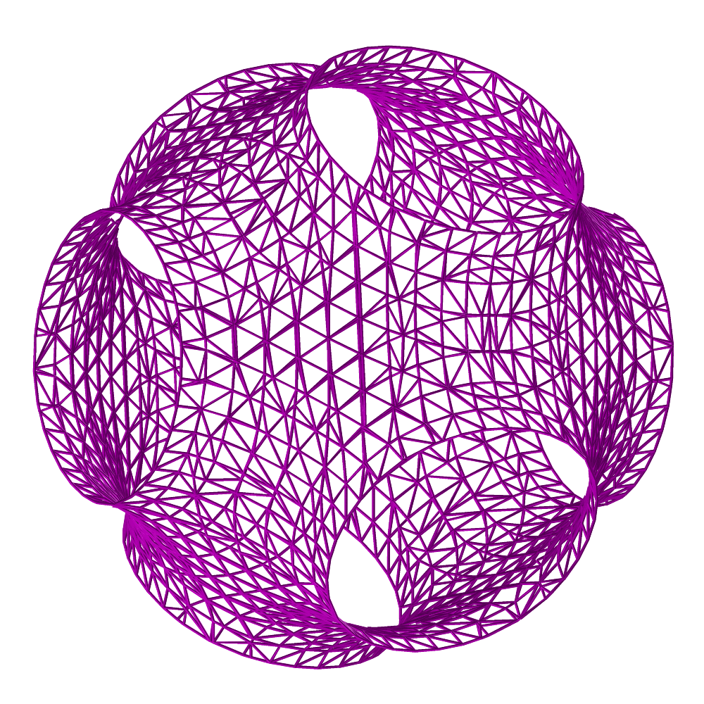
FIGURE:
The result of applying Marching Cubes to a trivariate scalar function
using the MRCHCUBE command.
MREFINE
MultivarType MREFINE( MultivarType TV, ConstantType Direction,
NumericType Replace, ListType KnotList )
provides the ability to Replace a knot vector of MV or refine
it in the specified direction Direction.
KnotList is a list of knots at which to refine MV. All knots should be
contained in the parametric domain of MV in Direction. If the knot
vector is replaced, the length of KnotList should be identical to the
length of the original knot vector of MV in Direction. If MV
is a Bezier multivariate, it is automatically promoted to be a B-spline
multivariate.
Example:
MV = MREFINE( MREFINE( MREFINE( MV,
0, FALSE, list( 0.333, 0.667 ) ),
1, FALSE, list( 0.333, 0.667 ) ),
2, FALSE, list( 0.333, 0.667 ) );
refines MV in the first three directions by adding two more knots at
0.333 and 0.667. See also CREFINE, SREFINE, and TREFINE.
MREGION
MultivarType MREGION( MultivarType MV, ConstantType Direction,
NumericType MinParam, NumericType MaxParam )
extracts a region of MV between MinParam and MaxParam
in the specified Direction. Both MinParam and MaxParam
should be contained in the parametric domain of MV in Direction.
Example:
MV1r1 = MREGION( MV1, 3, 0.1, 0.2 );
MV1r2 = MREGION( MV1, 3, 0.4, 0.6 );
MV1r3 = MREGION( MV1, 3, 0.99, 1.0 );
extracts three regions of MV1 along the 4th (directions are counted
from zero) direction. See also CREGION, SREGION, and TREGION.
MREPARAM
MultivarType MREPARAM( MultivarType MV, ConstantType Direction,
NumericType MinParam, NumericType MaxParam )
reparametrizes MV over a new domain from MinParam to MaxParam,
in the prescribed Direction. This operation does not affect the geometry
of the multivariate and only affine transforms its knot vectors. A Bezier
multivariate will automatically be promoted into a B-spline surface by this
function.
Example:
MV = MREPARAM( MREPARAM( MV, 0, 0.1, 1.9 ),
1, 0.1, 0.9 );
ensures that the multivariate MV is defined over [0.1, 0.9] in the first
two directions. See also CREPARAM, SREPARAM, and TREPARAM.
MREVERSE
MultivarType MREVERSE( MultivarType MV, NumericType Dir1, NumericType Dir2 )
reverses MV by flipping the given two parametric directions, Dir1
and Dir2, (starting to count directions from zero).
If, however, Dir2 is negative, the multivariate is reversed by flipping
the direction of MV in Dir1.
Example:
RevMV = MREVERSE( MV, 2, 4 );
reverses MV by flipping the third and fifth directions of MV.
See also SREVERSE and TREVERSE.
MSCIRC
CurveType MSCIRC( PolyType Poly, ListType Tols )
or
CurveType MSCIRC( ListType Geom, ListType Tols )
computes a minimum spanning circle to polyline(s) (first form), or to
a list of curves (second form).
Tols is a list of two numeric values, SubdivTol and NumerTol, that
are used only if the minimum spannng circle of a set of curves is required.
See MZERO for the meaning of the SubdivTol and NumerTol
tolerances.
The returned circle will have 'center' and 'radius' attributes with the
circles parameters. If a cone is returned, 'angle' and 'center' of the cone
will be returned.
Example:
Msc = MSCIRC( Crvs, list( 0.01, 1e-10 ) ):
See figure for minimum spanning circle of curves.
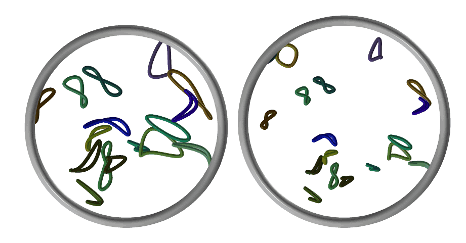
FIGURE:
The minimum spanning circle of a set of planar curves is computed with
the aid of MSCIRC. Two examples are shown.
MSCONE
ListType MSCONE( ListType Vecs )
computes the minimum spanning cone of a set of input vectors, Vecs.
Returned is a list of the cone's parameters as well as a geometry
representation of the cone.
Example:
MSC = MSCONE( Vecs );
See also MSCIRC and MSSPHERE
MSSPHERE
SurfaceType MSSPHERE( ListType Pts )
computes a minimum spanning sphere to a list of 3D points.
Returned is a geometric representation of the cone with "radius" and
"center" attributes of the parameters of the sphere.
Example:
MSS = MSSPHERE( Pts );
MUNIVZERO
ListType MUNIVZERO( ListType MVs, NumericType StepSize,
NumericType SubdivTol, NumericType NumerTol )
computes the simultaneous zeros of several scalar multivariate functions, in
MVs. The system is assumed to be underdetermined, having n constraints
in n+1 degrees of freedom (parameters).
StepSize specifies the marching step size.
SubdivTol specifies the subdivision tolerance in the
parametric domain of the multivariates, whereas NumerTol prescribes the
tolerance of the numerical improvement stage. A numerical improvement stage
is applied if |NumerTol| < SubdivTol. If NumerTol is
negative, and a numeric improvement stage is indeed applied, all points that
fail to improve to the requested accuracy are purged away.
A list of piecewise linear solution curves, each designating one univariate
in the parameter space of the multivariates, is returned.
Example:
UnivZeroMVs = MUNIVZERO( list( MV1, MV2, MV3 ), 0.01, -1e-6 );
See also SSINTR2, CONTOUR and MZERO.
MVCONTACT
MultivarType MVCONTACT( CurveType C1, CurveType C2, ListType MotionCrvs,
NumericType SubdivTol, NumericType NumerTol,
NumericType UseExprTrees )
or
MultivarType MVCONTACT( SurfaceType S1, SurfaceType S2, ListType MotionCrvs,
NumericType SubdivTol, NumericType NumerTol,
NumericType UseExprTrees )
computes the contact locations, if any, when C1 or S1 is
stationary and C2 or S2 is moving along the MotionCrvs
animation curves. Currently only "MOV_XYZ" and "SCL" animation curves are
supported.
SubdivTol and NumerTol control the tolerance of the computation
as in MZERO. If UseExpreTrees, expression trees are used in the
computation which is typically faster.
Example:
Cntct = MVCONTACT( s1, s2, list( mov_xyz ), 0.02, -1e-14, true );
MVEXPLICIT
MultivarType MVEXPLICIT( NumericType Dim, StringType Expression )
constructs a multivariate power basis from the given polynomial
Expression. The Expression can be any infix notational expression
using +-/*^ with no parenthesis. The parameters are the 26 letters A-Z.
The dimension of the multivariate is set by Dim and should be in line
with the variables used. A stands for the first dimension, B for the second,
etc., so if Dim equal 3, only A, B, and C could appear in Expression.
Having a higher letter with a lower dimension constitutes an error.
Example:
M1 = coerce( mvexplicit( 2, "A^2 + B^2 - 1" ), bezier_type );
M2 = coerce( mvexplicit( 2, "4 * A^2 + B^2 / 4 - 1" ), bezier_type );
constructs two scalar saddle Bezier bivariate surfaces, represented as
multivariates.
MVINTER
MultivarType MVINTER( ListType Geometry, NumericType SubdivTol,
NumericType NumerTol, NumericType UseExprTrees )
computes the intersection of two planar curves (Geometry is a list of
two planar curves) or three surfaces (Geometry is a list of three
surfaces).
SubdivTol and NumerTol control the tolerance of the computation
as in MZERO. If UseExpreTrees, expression trees are used in the
computation which is typically faster.
Example:
Sln1 = MVINTER( list( c1, c2 ), 0.001, 1e-8, true );
NCCNTRPATH
ListType NCCNTRPATH( PolyType Obj, NumericType Offset, NumericType ZBaseLevel,
NumericType TPathSpace, NumericType Units )
or
ListType NCCNTRPATH( SurfaceType Obj, NumericType Offset, NumericType ZBaseLevel,
NumericType TPathSpace, NumericType Units )
builds Numerically controlled (NC) tool path to mill (machine) the given Obj
geometry. The Offset prescribes the necessary offset, due to the tool's ball
end radius. ZBaseLevel sets a base level the toolpath will not go below.
and Units sets the used units with 0 for inches and 1 for mm. The toolpath
is built as parallel contours of the (offset of the) input Obj, contours that
are TPathSpace spacing apart.
The following attributes are optional and supported by NCCNTRPATH:
NCCntrBBox A string attribute with six numeric values as
"XMin XMax YMin YMax ZMin ZMax". Bounds the
working space of the contouring.
NCCntrClip A closed polyline object to clip the final
toolpath to be confined to its interior.
NCCntrMaxDepthStep Specifies how deep can tool plunge in compared
to the last depth, in the last contour. Adds
additional paths to confirm to this, if needed.
NCCntrSlowOnPlunge If set and plung this much, generates toolpath
with "RelFeedrate" attributes to slowdown.
Example:
Tea = load( "teapot" );
NCPath = NCCntrPath( Tea, 1/4, 0.0, 1/8, 0 );
attrib( NCPath, "NCRetractZLevel", 3.5 );
attrib( NCPath, "NCMaxXYBridgeGap", 0.25 );
save( "NCPath.nc", NCPath );
NC data can be saved using the SAVE command in G-code if the saved file type is
".nc". See SAVE for more, including the meaning of the different attributes in the
above example. See also NCPCKTPATH.
NCPCKTPATH
ListType NCPCKTPATH( PolyType Obj, NumericType ToolRadius, NumericType RoughOffset,
NumericType TPathSpace, NumericType TPathJoin,
NumericType Units, NumericType TrimSelfInters )
computes tool path to 2D pocket machining from +Z direction the given Obj
geometry (a closed curve or a closed polygon). ToolRadius sets the offset to
use in the pocket whereas RoughOffset sets the offset to use during roughing
(RoughOffset better be larger than ToolRadius). TPathSpace sets
the space between adjacent pockets slices in the zigzag motion and TPathJoin
prescribes the maximum distance to connect adjacent slices (if larger a full
retracting will be performed).
Units sets the used units with 0 for inches and 1 for mm and if
TrimSelfInters is TRUE also attempts to eliminate self intersections due
to the applied offsets.
Example:
TPath = NCPcktPath( Crv, 0.05, 0.06, 0.02, 0.05, 0, true );
attrib( TPath, "NCRetractZLevel", 1.0 );
attrib( TPath, "NCMaxXYBridgeGap", 0.05 );
save( "TPath.nc", TPath );
NC data can be saved using the SAVE command in G-code if the saved file type is
".nc". See SAVE for more, including the meaning of the different attributes in the
above example. See also NCCNTRPATH.
MZERO
ListType MZERO( ListType MVs, ListType Constraints,
NumericType SubdivTol, NumericType NumerTol )
computes the simultaneous zeros of several scalar multivariate functions, in
MVs.
Constraints is a list of positive, zero or negative values to denote
the respective constraint must be positive, zero or negative. Can be nil()
to denote all constraints are zero constraints.
SubdivTol specifies the subdivision tolerance in the parametric
domain of the multivariates, whereas NumerTol prescribes the tolerance
of the numerical improvement stage. A numerical improvement stage is applied
if |NumerTol| < SubdivTol. If NumerTol is negative,
and a numeric improvement stage is indeed applied, all points that fail to
improve to the requested accuracy are purged away.
A list of control points, each designating one location in the
parameter space of the multivariates, is returned.
The number of multivariates cannot exceed the dimension of the
multivariates. That is, if the MVs are trivariates, then, at most, three
of them may be provided. If less are provided, then the dimension of the
solution space is larger than zero and piecewise linear
univariates/bivariates/finite cloud of points sampled from that solution
space will be returned.
Example:
ZeroMVs = MZERO( list( MV1, MV2, MV3 ), nil(), 0.01, -1e-6 );
See also BFZEROS, CONTOUR and MUNIVZERO.
MPROMOTE
PromMV = MPROMOTE( MultivarType MV, ListType AddDir );
or
PromMV = MPROMOTE( MultivarType MV, ListType NewDimStartAxis );
promote the multivariate MV to a higher dimension. In the first form
(a list of one numeric value), the multivariate will be promoted to have one
more dimension (i.e. a bivariate would become a trivariate). The new added
axis will be AddDir.
The second form (a list of two numeric values) allows the original
multivariate to be placed at axes from StartAxis and have a new
dimensional NewDim.
Example:
ms = coerce( srf, multivar_type );
coerce( mfrommv( MPROMOTE( ms, list( 0 ) ), 0, 0.5 ), surface_type ) == srf;
coerces a surface to a multivariate, promotes it to a trivariate-multivariate,
extracts an iso-surface bivariate-multivariate along the new introduced axis
from the trivariate-multivariate and compares it to the original surface. It
should be equal!
NIL
ListType NIL()
creates an empty list so data can be accumulated in it.
See CINFLECT or CZEROS for examples. See also LIST and SNOC.
OFFSET
PolygonType OFFSET( PolygonType Poly, NumericType OffsetDistance,
NumericType Smoothing, NumericType MiterEdge )
or
CurveType OFFSET( CurveType Crv, NumericType OffsetDistance,
NumericType Tolerance, NumericType BezInterp )
or
CurveType OFFSET( CurveType Crv, CurveType OffsetDistance,
NumericType Tolerance, NumericType BezInterp )
or
SurfaceType OFFSET( SurfaceType Srf, NumericType OffsetDistance,
NumericType Tolerance, NumericType BezInterp )
or
TrimSrfType OFFSET( TrimSrfType TrimSrf, NumericType OffsetDistance,
NumericType Tolerance, NumericType BezInterp )
or
VoxelType OFFSET( VoxelType VxlMdl, NumericType OffsetDistance,
NumericType Tolerance, NumericType BezInterp )
offset Poly, Crv, Srf or a TrimSrf, by translating
all the vertices or control points in the direction of the normal of the
poly/curve or of the (trimmed) surface by an OffsetDistance amount.
For a Poly object, the input can be a single polygon or a single
polyline, in which case the offset is computed in the XY plane, or can be
a polygonal model in which case the offset is computed in R^3. In the
former case, the result is an offset of the original polygon/line
in the XY plane and is exact. In the latter case, the normals at the
vertices of the polygonal model are employed (and are locally estimated
if non detected), and all vertices are moved in the vertices normals,
scaled by this offset distance. For offset in R^3, if Smoothing
is TRUE, normals at the vertices are always recomputed and smoothed out.
Also for an offset in R^3, if MiterEdge is positive, attempts to
properly compenstate for miter edges' based offset is made, upto a scaling
factor set by the value of MiterEdge.
Otherwise, each control point has a node parameter value associated with
it, which is used to compute the normal. The returned curve or surface only
approximates the real offset. If the resulting approximation does not satisfy
the accuracy required by Tolerance, Crv or Srf or
TrimSrf is subdivided and an offset approximation fit is computed for
the two halves. For curves, one can request a Bezier interpolation scheme in
the offset approximation by setting BezInterp. BezInterp is
not yet supported for (trimmed) surfaces.
Negative OffsetDistance denotes offset in the reversed direction of the
normal.
If the curve is a 3D curve (E3 or P3) the offset is computed using the
nornal of the frenet frame of the curve. Make sure you use a 2D curve (E2 or
P2) for a proper offset in the plane.
If OffsetDistance is a (scalar) curve, the curve's first coordinate
is used to prescribe a variable offset amount along the curve for which we
compute the variable offset. Both Crv and OffsetDistance must share
the same parametric domain.
In the case of input that is VoxelType, the OffsetDistance is
measured in pixels and Tolerance and BezInterp are ignored.
Example:
OffCrv = OFFSET( Crv, -0.4, 0.1, off );
offsets Crv by the amount of -0.4 in the reversed normal direction,
Tolerance of 0.1 and no Bezier interpolation.
See also TOFFSET, AOFFSET, LOFFSET and MOFFSET.
See figure for an example.
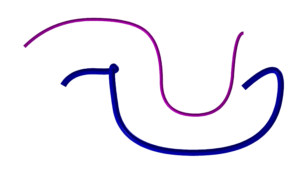
FIGURE:
Offset approximation (thick) of a B-spline curve (thin).
ORTHOTOMC
CurveType ORTHOTOMC( CurveType Crv, PointType Pt, NumericType K )
or,
SurfaceType ORTHOTOMC( SurfaceType Srf, PointType Pt, NumericType K )
compute the K-orthotomic of freeform curves and surfaces. See
Fundamentals of Computer Aided Geometric Design, by J. Hoschek and
D. Lasser.
Example:
pt = point( 0, 0.35, 0 );
crv = cbezier( list( ctlpt( E2, -0.8, -0.6 ),
ctlpt( E2, -0.3, -0.2 ),
ctlpt( E2, 0.0, 0.0 ),
ctlpt( E2, 0.8, -0.6 ) ) );
Orth = ORTHOTOMC( crv, pt, 2 );
interact( list( Orth, crv, pt ) * tx( 0.5 ) ) );
computes the orthotomic of a cubic Bezier curve that has an inflection
point. Note that inflection points are reduced to cusps in the orthotomic
result.
See figure for an example.
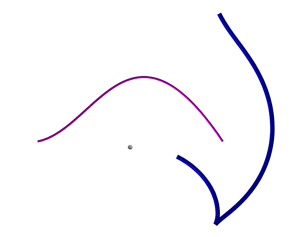
FIGURE:
An orthotomic (thick) of a cubic Bezier curve. The inflection
point in the cubic Bezier is reduced to a cusp in the orthotomic.
Computed using the ORTHOTOMC command.
PATTRIB
AnyType PATTRIB( PolyType Poly, NumericType Index,
StringType Name, AnyType Value )
provides a mechanism to set/get an attribute to a vertex of a polygon.
Unlike the regular ATTRIB/RMATTR functions, PATTRIB allows access to the
Index vertex in polygon Poly, access that is otherwise impossible.
Index starts at zero for the first vertex.
The attribute will have a name Name and a value Value. If Value
is NIL(), no attributes are set and the named attribute, if any, is returned.
This PATTRIB function only allows numeric values or strings as Value.
For example,
PATTRIB( Tri, 0, "rgb", "255,0,0");
PATTRIB( Tri, 1, "rgb", "0,255,0");
PATTRIB( Tri, 2, "rgb", "0,0,255");
sets the RGB values of the three vertices of triangle Tri.
See also PNORMAL, ATTRIB, ATTRPROP, GETATTR, RMATTR, CPATTR, FINDATTR.
PCIRCLE
CurveType PCIRCLE( VectorType Center, NumericType Radius )
is the same as CIRCLE but approximates the circle as a polynomial curve.
See also CIRCLE.
PCIRCAPX
CurveType PCIRCAPX( VectorType Center, NumericType Radius, NumericType Order,
NumericType Continuity, NumericType Tol )
is the same as CIRCLE but approximates the circle as a polynomial curve
of a specific tolerance. Order can be either 3 or 4 for a qudaratic or
a cubic approximation, Continuity governs the continuity between the
different polynomial arcs and can be 0 (for C^0) or 1 (for C^1), and Tol,
that governs the accuracy of the constructed approximated circle, can be any
accuracy up to around 10^-15.
c = PCIRCAPX( vector( 0, 0, 0 ), 1, 3, 1, 1e-6 ):
constructs a quadratic polynomial circe approximation with tolarenace 1e-6.
See also CIRCLE and PCIRCLE.
PCRVTR
PolyType PCRVTR( PolyType Pl, NumericType NumOfRings, NumericType CubicFit )
estimates curvature properties of given polygonal model Pl, assuming
Pl originated from a continuous freeform surfaces. NumOfRings
sets the number of rings around a vertex that will be used to estimate the
curvature properties of the vertex. If (CubicFit is TRUE, a cubic
fit is computed to the local vertex neighborhood, or a quadratic fit, if
FALSE.
The return polygonal object is identical to Pl, but with the
following attributes set at each vertex:
"K1Curv" First principal curvature value
"K2Curv" Second principal curvature value
"KCurv" The Gaussian Curvature
"HCurv" The Mean Curvature
"D1" The first principal direction
"D2" The second principal direction
See also PPROPFTCH.
PDOMAIN
ListType PDOMAIN( FreeformType Freeform )
returns the parametric domain of the given Freeform.
See also MESHSIZE, FFCTLPTS, FFKNTVEC, FFMESH, FFMSIZE, FFPTTYPE, FFORDER.
Example:
circ_domain = PDOMAIN( circle( vector( 0.0, 0.0, 0.0 ), 1.0 ) );
PINTERP
PlaneType PINTERP( ListType PtsList )
least squares fits a plane to a given set of points PtsList.
Example:
Pln = PINTERP( Pts );
PIMPRTNC
PolyType PIMPRTNC( PolyType Pl, NumericType GenImprtncPolylines )
computes the importance of a local neighborhood in a triangular polygonal
mesh Pl, based on the dihedral angles of the edges in that neighborhood.
If GenImprtncPolylines FALSE, every vertex in the returned mesh will
have a "SilImp" (See the connection of this importance to silhouettes?)
attribute with its importance. Otherwise, if GenImprtncPolylines TRUE,
polylines that stylistically convey the importance of the different regions
in this mesh are returned.
Example:
Pl = triangl( box( vector( 0, 0, 0 ), 1, 2, 3 ), 1 );
PlImp = PIMPRTNC( Pl, 0 );
PLANE
PointType PLANE( NumericType A, NumericType B, NumericType C, NumericType D )
creates a plane type object, using the four provided NumericType
coefficients. See also VECTOR, POINT.
PLANECLIP
ListType PLANECLIP( PolyType Poly, PlaneType Pln )
clips a polygonal model Poly against a plane Pln.
Three polygonal objects are returned in a list: polygons on the positive side
of the plane, polygons that intersect the plane, and polygons on the negative
side of the plane, in this order.
If one of these lists is empty, a numeric zero is substituted.
Example:
Pls = PLANECLIP( Pl, plane( 1, 1, 0, 0 ) );
clips polygonal object Pl against the plane X+Y=0.
PLN3PTS
PlaneType PLN3PTS( PointType Pt1, PointType Pt2, PointType Pt3 )
computes a plane out of three points.
Example:
Pl1 = PLN3PTS( point( 0, 0, 0 ), point( 0, 1, 0 ), point( 1, 0, 0 ) );
PLYROUND
PlaneType PLYROUND( NumericType RoundMethod, PolyType Mesh,
PolyType Edge, ListType Params )
or
PlaneType PLYROUND( NumericType RoundMethod, ListType TwoMeshes,
PolyType Edge, ListType Params )
apply a arounding to Mesh or TwoMeshes along the prescribed
Edge, or in the entire mesh(es) if Edge nil(). Params sets the
different parameters of the roundings, depending on the value of
RoundMethod:
If RoundMethod is 1, the rounded area is locally smoothed out by
local averaging in the neighborhood of the Edge. Then, Params
is a list of the form
(SmoothNormals, NumIterations, RoundPower, AllowBndryMove, RoundingRadius)
where if SmoothNormals TRUE we also estimate smooth normals,
NumIterations controls how many smoothing iterations to apply,
RoundPower controls the decay power as we get away from the Edge,
AllowBndryMove allows the boundary to freely move if -1, allows the
boundary to move only along the plane containing the boundary curve if 1,
and fixes the boundary if 0.
RoundingRadius sets the (approximated) rounding radius.
If RoundMethod is 3, the rounded area is locally projected onto a
rounded swept geometry in the neighborhood of the Edge. Then,
Params is a list of the form
(moothNormals, RoundRadius, RoundPower)
where if SmoothNormals TRUE we also estimate smooth normals,
RoundingRadius sets the (approximated) rounding radius, and
RoundPower controls the decay power as we get away from the Edge.
Other values of RoundMethod are not allowed and in no case, the
result is a perfect circular rounding.
Example
RPlns1 = PlyRound( 1, Pln, nil(), list( TRUE, 100, 1.0, 0, 0.1 ) ):
RPlns2 = PlyRound( 1, Pln, Edge, list( TRUE, 10, 1.0, 1, 0.5 ) ):
rounds poly mesh Pln twice. Once into RPlns1, rounding the
entire mesh by smoothing in 100 iterations and fixing the boundary, and
once into RPlns21, rounding only along edge Edge, in 10
iterations and boundary can move only along the plane holding the boundary.
PMORPH
PlaneType PMORPH( PolyType Pl1, PolyType Pl2, NumericType Blend )
creates a new polygonal object which is a metamorph of the two given
polygonal objects that share the same topology. That is, Pl1 and Pl2
must share the same number of polygons and the i'th polygon in Pl1 must
be equal in its number of vertices to the i'th polygon of Pl2.
This is very useful if a sequence that "morphs" one polygonal model to
another is to be created.
Example:
Pl1 = con2( vector( 0.0, -0.5, -0.5 ), vector( 0.0, 0.0, 1.0 ), 0.4, 0.1, 3 );
Pl2 = con2( vector( 0.0, 0.5, 0.0 ), vector( 0.0, 0.0, 1.0 ), 0.1, 0.4, 3 );
Pl = PMORPH( Pl1, Pl2, 0.5 );
creates a cylinder out of two truncated cones, using PMORPH. See also
CMORPH and SMORPH.
PNORMAL
PointType PNORMAL( PolyType Poly, NumericType Index, VectorType Normal )
provides a mechanism to set/get the normal of vertex number Index
in a polygon Poly. Index starts at zero for the first vertex.
Normal replaces the current normal that is also returned. If
Normal is not a VectorType, no new normal is set but the current
normal is still returned, allowing normals to be queried.
For example,
PNORMAL( Tri, 0, vector( 1, 0, 0 ) );
PNORMAL( Tri, 1, vector( 0, 1, 0 ) );
sets the normals of the first two vertices in triangle Tri to be
the X and Y axes, respectively.
See also PATTRIB.
POINT
PointType POINT( NumericType X, NumericType Y, NumericType Z )
Creates a point type object, using the three provided NumericType scalars.
See also VECTOR, PLANE.
POLARSIL
PolygonType POLARSIL( SurfaceType Srf, VectorType ViewDir,
NumericType SubdivTol, NumericType EuclideanSpace )
Computes the polar silhouettes of surface Srf from view direction
ViewDir. Equal to < S(u, v) x N(u, v), VDir > = 0. If
EuclideanSpace TRUE, the polar silhouettes are returned in Euclidean
space, over Srf. Otherwise, the polar silhouettes are returned in the
parametric domain of Srf. SubdivTol controls the accuracy of the
computation of the polar silhouettes.
Example:
pSil = polarsil( glass, vector( 1, 0, 0 ), 0.01, true );
See figure for this example.
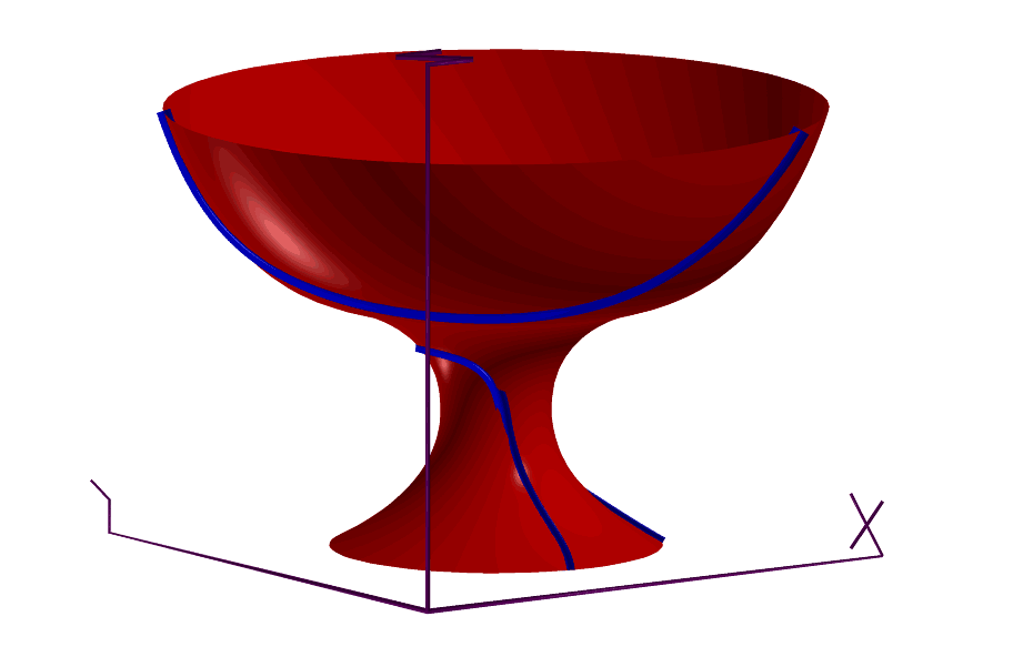
FIGURE:
Polar silhouette computed for this glass shaped surface using the
POLARSIL
POLY
PolygonType POLY( ListType VrtxList, NumericType IsPolyline )
creates a single polygon/polyline (and therefore open) object, defined by
the vertices in VrtxList (see LIST). All elements in VrtxList
must be one of PointType, VectorType, CtlPtType, or PolygonType types.
If IsPolyline, a polyline is created; otherwise, a polygon.
Example:
V1 = vector( 0.0, 0.0, 0.0 );
V2 = vector( 0.3, 0.0, 0.0 );
V3 = vector( 0.3, 0.0, 0.1 );
V4 = vector( 0.2, 0.0, 0.1 );
V5 = vector( 0.2, 0.0, 0.5 );
V6 = vector( 0.3, 0.0, 0.5 );
V7 = vector( 0.3, 0.0, 0.6 );
V8 = vector( 0.0, 0.0, 0.6 );
V9 = vector( 0.0, 0.0, 0.5 );
V10 = vector( 0.1, 0.0, 0.5 );
V11 = vector( 0.1, 0.0, 0.1 );
V12 = vector( 0.0, 0.0, 0.1 );
I = POLY( list( V1, V2, V3, V4, V5, V6, V7, V8, V9, V10, V11, V12 ),
FALSE );
constructs an object with a single polygon in the shape of the letter I.
See figure for an example.

FIGURE:
Polygons or polylines can be manually constructed using the
POLY constructor.
POLYMESH2TV
TrivarType POLYMESH2TV( PolygonType Mesh, PolygonType MedAxis,
NumericType MeanErr, HausdErr )
Fits a trivariate to a given tube-like poly geometry Mesh.
The input should also include MedAxis - a medical axis rough
approximation of the to-be-constructured tube-like trivariates.
The last two parameters MeanErr and HausdErr, contol
the allowed mean and Hausdorff errors in the fit.
Example:
TV = POLYMESH2TV( Mesh, Pls, 0.01, 0.02 );
POLYHOLES
PolygonType POLYHOLES( PolygonType OuterPoly, PolygonType Island )
or
PolygonType POLYHOLES( PolygonType OuterPoly, ListType Islands )
merges the given Island(s) into the main polygon OuterPoly,
creating a polygon with holes. The outer polygon OuterPoly is assumed
to be oriented in the opposite direction to that of the Island(s).
PPINCLUDE
NumericType PPINCLUDE( PolyType Pl, PointType Pt )
tests if a point Pt is inside a 3D closed polyhedra Pl in 3-space
or if a point Pt is inside a 2D closed polygon Pl in 2-space, if
Pl contains only one (planar) polygon.
Returns TRUE if inside, FALSE otherwise.
Example:
if ( PPINCLUDE( Pl, pt ),
... );
See also CPINCLUDE.
PPINTER
ListType PPINTER( PolyType Pl1, PolyType Pl2 )
computes the intersection of two individual polygons in R3, Pl1 and
Pl2. Similar results can also be obtained via Boolean operations.
Example:
Pl1 = poly( list( point( -1, -1, 0 ),
point( -1, 1, 0 ),
point( 1, 1, 0 ),
point( 1, -1, 0 ) ), false );
Pl2 = Pl1 * rx( 70 ) * tx( 0.5 );
Inter1 = PPINTER( Pl1, Pl2 );
iritstate( "intercrv", true );
Inter2 = Pl1 * Pl2;
computes the intersection edge of two polygons in two different ways. Note,
however, that while PPINTER considers only the first polygon in a
polygonal object, the Boolean operations considers them all.
PPROPFTCH
PolyType PPROPFTCH( PolyType Pl, NumericType PropType, ListType PropParam )
computes piecwise linear curves over polygonal mesh Pl. The extracted
curves could be one of,
Property PropType PropParam
Attribute Value 0 list( AttrName, AttrValue )
Isophotes 1 list( ViewDir, InclinationAngle )
Gaussian Crvtr 2 list( NumRingCrvtrAprx, CrvtrVal )
Mean Crvtr 3 list( NumRingCrvtrAprx, CrvtrVal )
The NumRingCrvtrAprx specifies how many rings around a vertex should be
considered when the curvature of the vertex is estimated. Typically 1.
Example:
Pl1 = PPropFtch( Srf, 1, list( normalize( vector( 1, 1, 1 ) ), 90 ) );
Pl2 = PPropFtch( Srf, 1, list( normalize( vector( 1, -1, 1 ) ), 90 ) );
Pl3 = PPropFtch( Srf, 1, list( normalize( vector( 1, 0, 1 ) ), 90 ) );
extracts silhouettes from surface Srf (note an InclinationAngle of 90
degrees extract silhouettes), from three different viewing direction.
See also PCRVTR, SILHOUETTE, ISOCLINE, PPROPFTCH and SASPCTGRPH.
PRINTER
ListType PRINTER( PolyType Pl, NumericType RayPt, NumericType RayDir )
computes the number of XY planar intersection of ray (RayPt, RayDir)
with a single polygon Pl. Returned is the number of interesections
found.
PRISA
ListType PRISA( SurfaceType Srfs, NumericType SamplesPerCurve,
NumericType Epsilon, ConstantType Dir, VectorType Space,
NumericType CrossSecs )
or
ListType PRISA( TrimSrfType TrimSrfs, NumericType SamplesPerCurve,
NumericType Epsilon, ConstantType Dir, VectorType Space,
NumericType CrossSecs )
compute a layout (prisa) of the given surface(s) Srfs or TrimSrfs,
and return a list of (trimmed) surface objects representing the layout.
The surface is approximated to within Epsilon in direction Dir
into a set of ruled surfaces, and then developable surfaces that are laid out
flat onto the XY plane. If Epsilon is negative, the piecewise ruled
surface approximation in 3-space is returned.
SamplesPerCurve controls the piecewise linear approximation of the
boundary of the ruled/developable surfaces. Space is a vector whose
X component controls the space between the different surfaces' layout, and
whose Y component controls the space between different layout pieces.
If CrossSecs is not zero, the 3D cross sections, approximated as
planar, of each laid out region are also provided.
Example:
cross = cbspline( 3,
list( ctlpt( E3, 0.7, 0.0, 0. ),
ctlpt( E3, 0.7, 0.0, 0.06 ),
ctlpt( E3, 0.1, 0.0, 0.1 ),
ctlpt( E3, 0.1, 0.0, 0.6 ),
ctlpt( E3, 0.6, 0.0, 0.6 ),
ctlpt( E3, 0.8, 0.0, 0.8 ),
ctlpt( E3, 0.8, 0.0, 1.4 ),
ctlpt( E3, 0.6, 0.0, 1.6 ) ),
list( KV_OPEN ) );
wglass = surfrev( cross );
wgl_ruled = PRISA( wglass, 6, -0.1, COL, vector( 0, 0.25, 0.0 ), false );
wgl_prisa = PRISA( wglass, 6, 0.1, COL, vector( 0, 0.25, 0.0 ), true );
computes a layout of a wine glass in wgl_prisa and a three-dimensional
ruled surface approximation of wglass in wgl_ruled.
See figure for an example.
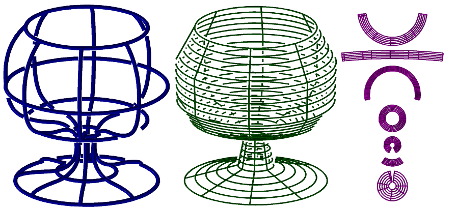
FIGURE:
The layout (prisa in hebrew...) of a freeform surface can be approximated
using the PRISA function.
See also PRULEDALG.
PSUBDIV
CurveType PSUBDIV( PolyType Plgns, NumericType SubdivisionScheme,
NumericType Numiterations, NumericType SmoothNormals,
NumericType TrianglesOnly, NumericType AdditionalParam )
applies one of several subdivision schemes to the given polygonal object
Plgns. The SubdivisionScheme can be one of: Catmull Clark if 0,
Loop if 1, Butterfly if 2.
The number of subdivision iterations applied is set by Numiterations.
If SmoothNormals is TRUE, a normal approximation scheme is applied
to the result, for the vertices of the model, by averaging adjacent faces
normals at each vertex.
If TrianglesOnly, the output is examined and non triangles are
dividied into triangles.
Finally, if the Butterfly scheme is applied, AdditionalParam is
used as the tension.
CatmulRomPl = PSUBDIV( Plgns, 0, 1, 1, 1, 0 );
See figure for an example.
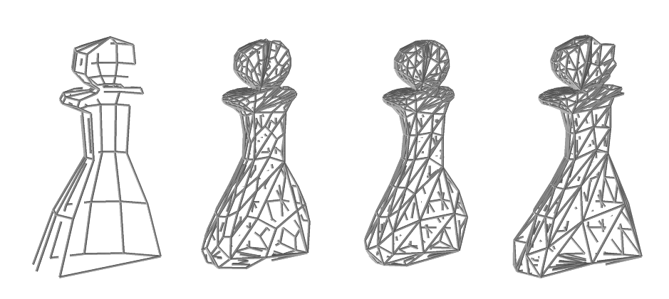
FIGURE:
Applied a subdivision scheme for polygonal models using the
PSUBDIV command. From left to right: Original half-a-pawn model,
Catmull Clark, Loop, and Butterfly, after one iteration.
PT3BARY
VectorType PT3BARY( PointType Pt1, PointType Pt2, PointType Pt3,
PointType InteriorPt )
computes the barycentric coordinates of InterPt with respect
to the triangle defined by Pt1, Pt2, Pt3.
A vector of three coefficents, which are the weights of the three
points of the triangle, are returned. InteriorPt is assumed to be in the
triangle.
Example:
Coeffs = PT3BARY( point( 0, 0, 0 ),
point( 1, 0, 0 ),
point( 0, 1, 0 ),
point( 0.25, 0.25, 0.0 ) );
PTHMSPR
ListType PTHMSPR( NumericType Size )
computes a fairly uniform distribution of points on a hemisphere.
Size hints at the distance between adjacent placed points.
Example:
Pts = PTHMSPR( 0.1 );
PTLNPLN
VectorType PTLNPLN( PointType LineOrig, VectorType LineRay, PlaneType Plane )
computes the point of intersection of given line LineOrig,
LineRay with plane Plane.
Example:
InterPt = PtLnPln( point( 1, 0, 1 ), vector( 1, 1, 1 ), Plane( 0, 0, 1, 0 ) );
PTPTLN
VectorType PTPTLN( PointType Point, PointType LineOrig, VectorType LineRay )
computes the point on line LineOrig, LineRay that is closest
to point Point. See also DSTPTLN.
Example:
ClosestPt = PTPTLN( point( 0, 0, 0 ), point( 1, 1, 0 ), vector( 1, 1, 1 ) );
PTREGISTER
MatrixType PTREGISTER( ListType PtSet1, ListType PtSet2,
NumericType StepSize, NumericType Tolerance )
registers one points set, PtSet1, with another, PtSet2.
The two points sets are assumed to be rigid motion of one another.
StepSize controls the step size of the numerical process and must be
a positive real less than 1.0. The larger StepSize is, the faster the
convergance with less stability. Finally, Tolerance prescribes the
necessary accuraacy in L-infinity sense. This function will converge for
small rotational deviations only.
Pt1 = nil();
for (i = 0, 1, 15,
Pt = point( random( -.7, .7 ), random( -.7, .7 ), random( -.7, .7 ) ):
snoc( Pt * tx( 0 ), Pt1 ) );
Pt2 = Pt1 * rx( 13 ) * ry( 5 ) * rz( 11 )
* tx( 0.1 ) * ty( 0.03 ) * tz( -0.05 );
Tr = PTREGISTER( Pt1, Pt2, 1, 1e-6 );
PTS2PLLN
ListType PTS2PLLN( ListType Points, NumericType MaxMatchDist )
matches the given cloud of points in a list of polylines.
MaxMatchDist is used as the maximal distance between two adjacent
points to connect.
Example:
Pts = nil();
for ( i = 0, 1, 100,
t = random( 0, 2 * Pi ):
snoc( point( cos( t ), sin( t ), 0 ), Pts ) );
Pll = PTS2PLLN( Pts, 0.1 );
connects 100 random points on the unit circle into a polyline
approximating an (almost) complete circle.
PTS2PLYS
PolylineType PTS2PLYS( ListType Points, NumericType MergeTol )
merges a list of points Points to polylines. Merges the points until
two adjacent points are at most MergeTol apart. Points is a list
of with PointType or CtlPtType. In the later case the control point can be of
arbitrary dimension.
PTSLNLN
ListType PTSLNLN( PointType Line1Orig, VectorType Line1Ray,
PointType Line2Orig, VectorType Line2Ray )
computes the closest two points on the two lines defined by point
LineiOrig and ray LineiRay. See also DSTLNLN.
A list object with the two points is returned.
Example:
ClosestPts = PtsLnLn( point( 1, 0, 0 ), vector( 0, 1, 0 ),
point( 0, 1, 0 ), vector( 1, 0, 0 ) );
QUADCRVS
ListType QUADCRVS( CurveType Crv, NumericType Tolerance, NumericType MaxLen )
approximates given curve Crv using piecewise quadratic curves upto
the prescribed tolerance Tolerance. If MaxLen is positive it
is used to limit the arc length of the cubic curves segments.
Example:
PQaudCrv = QUADCRVS( Crv, 0.01, 0.5 );
creates a piecewise quadratic approximation to curve Crv upto tolerance
0.01 and maximal arc length of cubic segments of 0.5.
See also CUBICCRVS, CBIARCS.
QUADRIC
ListType QUADRIC( ListType ABCDEFGHIJ ) )
or
ListType QUADRIC( ListType ABCDEFZ ) )
in the first form, constructs a quadric parametric surface whose
coefficients are the ten coefficients in the list ABCDEFGHIJ:
A x^2 + B y^2 + C z^2 + D xy + E xz + F yz + G x + H y + I z + J = 0.
In the second form, promotes the given conic curve whose coefficients
are the first six coefficients in the list ABCDEFZ:
A x^2 + B xy + C y^2 + D x + E y + F = 0.
into a quadric surface with height in z of Z amount, the seven'th list
element.
Example:
Sph = QUADRIC( list( 1, 1 , 1 , 0, 0, 0, 0, 0, 0, -1 ) );
Hyp1s = QUADRIC( list( 1, 1, -1, 0, 0, 0, 0, 0, 0, -1 ) );
Hyp2s = QUADRIC( list( 1, -1, -1, 0, 0, 0, 0, 0, 0, -1 ) );
Ellipse = list( 1, 0, 2, 0, 0, -1 ):
Ellipsoid = QUADRIC( Ellipse + list( 0.1 ) );
constructs four quadric surfaces, a sphere, a portion of a hyperboloid of
one sheet, a portion of a hyperboloid of two sheets, and promotes an
ellipse to an ellipsoid of Z height of 0.1.
Note only elliptic surfaces are compact and are reconstructed in whole.
Because the parametrization of the quadric is predetermined, one might need
to use SREGION and SMOEBIUS to extract subregions and/or reparametrize the
surface.
See also CONICSEC, IMPLCTTRANS, ELLIPSE3PT.
RAYTRAPS
ListType RAYTRAPS( ListType Crvs, NumericType Orient
NumericType SubdivTol, NumericType NumerTol,
NumericType UserExprTree )
or
ListType RAYTRAPS( ListType Srfs, NumericType Orient
NumericType SubdivTol, NumericType NumerTol,
NumericType UserExprTree )
computes locations on the given planar curves or 3-space surfaces that
would bounce rays from one object to the next, in an infinite cycle. Such
traps are denoted ray traps. Ray-traps are computed for the given list
of Crvs or Srfs, in the given order. The ray-trap problem is
posed as a set of n multivariate algebraic constraints with n variables,
given n objects prescribed in Crvs or Srfs. The simultaneous
solution of these constraints is computed using the MZERO function. See
MZERO for the meaning of the SubdivTol and NumerTol tolerances.
If Orient, attempt is made to orient the curves/surfaces which is
likely to speed up the process. If UserExprTree, expression trees
constraints are used instead of tensor products. Again, typically faster
and much less memory use.
Example:
Crv1 = pcircle( vector( -0.75, -0.75, 0 ), 0.5 );
Crv2 = Crv1 * sc( 1.5 ) * tx( 2 );
Crv3 = Crv1 * sc( 0.5 ) * tx( 0.2 ) * ty( 0.6 );
Tris = RayTraps( list( Crv1, Crv2, Crv3 ), 0.1, -1e-6 );
computes the ray-traps between three circles.
See figure for an example.
FIGURE:
Computes all ray-traps between three circles, using RAYTRAPS.
RFLCTLN
ListType RFLCTLN( SurfaceType Srf, VectorType ViewDir,
ListType LinesSprs, NumericType Euclidean )
computes reflection lines/ovals to the given surface Srf as
seen from view direction ViewDir. The resulting piecewise linear
curves are in Euclidean space if Euclidean is TRUE and in Srf
parameter space, otherwise.
The reflection/ovals themselves are defined via LinesSprs.
For reflection lines, LinesSprs consists of
list( LineDir, list( LinePos1, LinePos2, ... , LinePosN ) );
defining n parallel lines with direction LineDir through
point LinePos1 to LinePosN.
For reflection ovals, LinesSprs consists of
list( SprCntr, list( Rad1, Rad2, ... , RadN ) );
defining n co-spherical spheres, all located at SprCntr with
radii of Rad1 to RadN.
Example:
resolution = 20;
RefLns = RflctLn( Srf,
vector( 0, 1, 2 ),
list( vector( 0, 0, 1 ),
list( point( -3.0, 2, 0 ),
point( -1.5, 2, 0 ),
point( 0.0, 2, 0 ),
point( 1.5, 2, 0 ),
point( 3.0, 2, 0 ) ) ),
true );
RefOvals = RflctLn( Srf,
vector( 1, 1, 0 ),
list( point( 0, 2, 0 ),
list( 5, 25, 45, 65, 85 ) ),
true );
computes the reflection lines of surface Srf from viewing
direction ( 0, 1, 2 ) having five reflected lines and computes five
reflection ovals from viewing direction ( 1, 1, 0 ).
See also ReflectLns attributes in the display devices.
ROCKETFUEL
ListType ROCKETFUEL( SurfaceType SectionSrfGeom, VectorType MeshSize,
CurveType ThurstProfileCurve, NumericType SliceThrough,
NumericType BndrySrfs, NumericType ApplyRGB )
or
ListType ROCKETFUEL( TrivarType TVGeom, VectorType MeshSize,
CurveType ThurstProfileCurve, NumericType SliceThrough,
NumericType BndrySrfs, NumericType ApplyRGB )
computes an abstract hetergeneous rocket fuel based on a given geometry,
that can either be a cross section surface, SectionSrfGeom, to be
rotated along Zto form a trivariate, or a trivariate directly, as
TVGeom. The volumetric geometry is sampled MeshSize samples
in (u, v, w), during the approximation. The buring profile is set via
ThurstProfileCurve, with a time domain of [0, 1], where the last
dimension of ThurstProfileCurve is used as the buring rate.
The last three parameters controls the output. if SliceThrough
is TRUE, some portion of the volume is removed to show the inside. If
BndrySrfs is TRUE, the boundary surfaces of the volume are returned
(i.e. for fast display) instead of the full volumetric geometry. Both
returned surfaces or trivariates are going to be in E4 or P4 space, where
the fourth dimension specifies the amount of retardant (negative) or
accelerants (positive) to relatively locally add. Finally, if
ApplyRGB is TRUE, "rgb" attributes are added to the geometry
according to the heterogeneity mix, have retardants in blue, accelrant
in red and nuetral fuel in green.
Example:
Fuel = rocketFuel( TV, vector( 10, 10, 10 ), ThrustCurve,
TRUE, TRUE, TRUE );
generates the abstract fuel shaped as trivariate TV, sampled into
a 10x10x10 grid, having a thrust profile following ThrustCurve,
with a slice through the geometry of the result, with boundary surfaces
only, and RGB colors representing the heterogeneity.
RRINTER
ListType RRINTER( CurveType Srf1Crv1, CurveType Srf1Crv2,
CurveType Srf2Crv1, CurveType Srf2Crv2,
NumericType SubdivTol, NumericType ZeroSetFunc )
computes the intersection curves of the given two ruled surfaces,
defined as
SrfiCrv1 * v + SrfiCrv2 * (1 - v)", i = 1, 2, v in [0,1].
The ruled ruled intersection (RRI) problem is tranformed into a zero set
finding on another function. If ZeroSetFunc is true, the function
whose zero set provides the RRIsolution is returned. Otherwise, if
ZeroSetFunc is false, the RRI solution itself is returned. The zero
set is computed via numerical zero set finding methods and Tolerance
controls the fineness of the approximated solution. If Tolerance is
negative, the absolute value is employed as Tolerance but the
intersection curves are computed as if the two ruled surfaces are infinite
(i.e. v is unbounded).
See figure for an example.
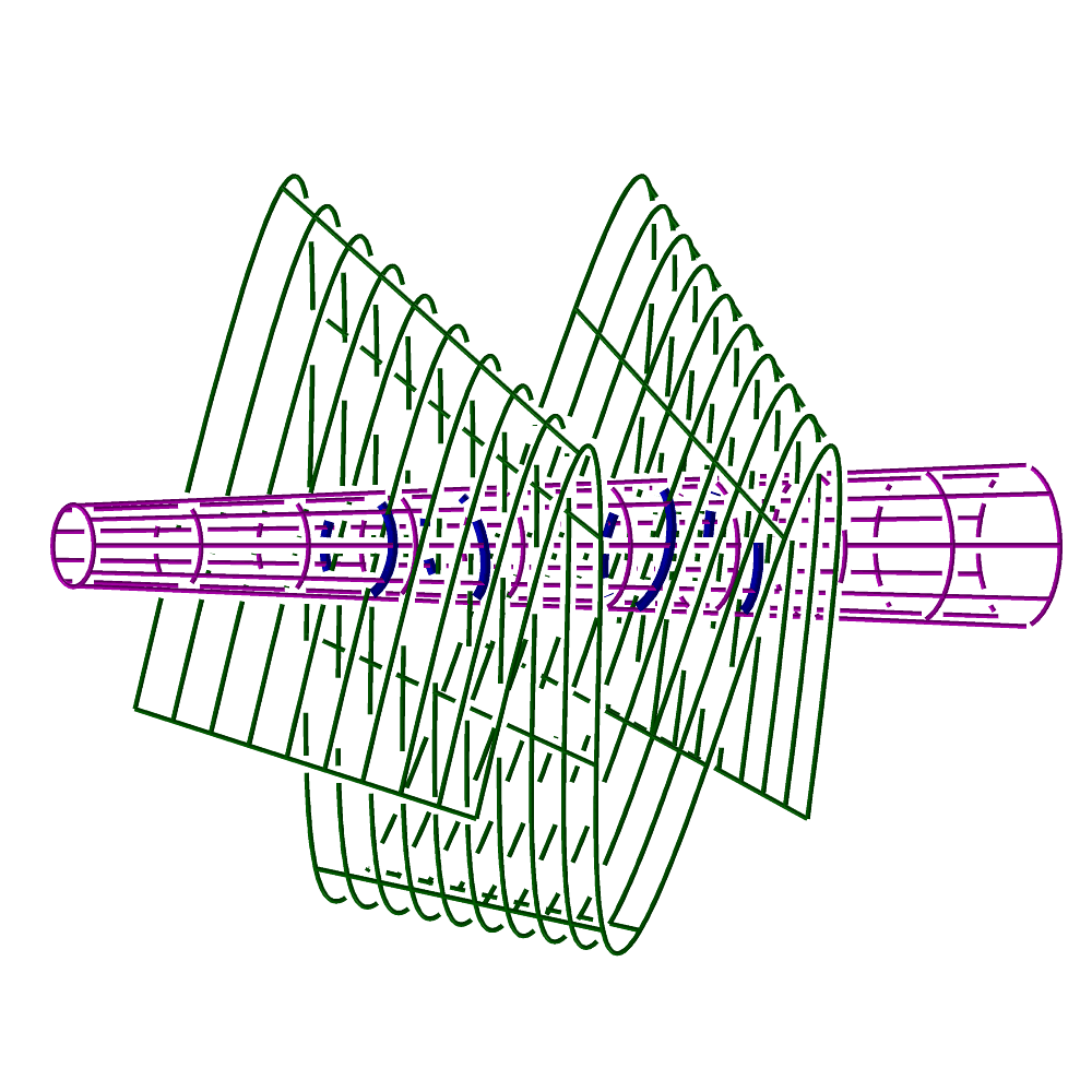
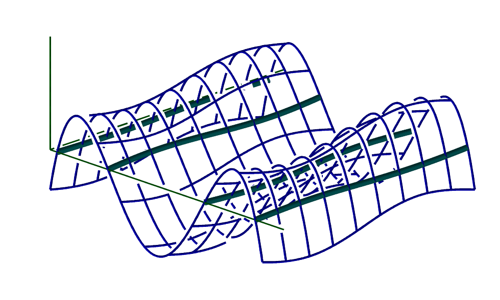
FIGURE:
Computation of the intersection curve between two ruled surfaces via
the RRINTER command. On the left, the four intersection curves are
shown, while (right) shows the computed function whose zero set
provides the request RRI solution.
Example:
c1 = cbezier( list( ctlpt( E3, -1.0, -1.0, -1.0 ),
ctlpt( E3, -0.5, 8.0, -1.0 ),
ctlpt( E3, 0.0, -15.0, -1.0 ),
ctlpt( E3, 0.5, 8.0, -1.0 ),
ctlpt( E3, 1.0, -1.0, -1.0 ) ) );
c2 = c1 * sc( 0.7 ) * tz( 1.7 );
r1 = ruledSrf( 0, c1, c2 );
c1 = pcircle( vector( 0, 0, 0 ), 0.3 ) * tz( 2 );
c2 = c1 * sc( 0.5 ) * tz( -3 );
r2 = ruledSrf( 0, c1, c2 ) * ry( 90 );
c = RRINTER( cMesh( r1, row, 0 ),
cMesh( r1, row, 1 ),
cMesh( r2, row, 0 ),
cMesh( r2, row, 1 ),
0.1, false );
interact( list( r1, r2, nth( c, 1 ) ) );
See also SSINTER, SSINTR2 and GGINTER.
RULEDFIT
SurfaceType RULEDFIT( SurfaceType Srf, NumericType Dir,
NumericType DomainExtension, NumericType SamplingRate )
fits a ruled surface to the given general surface Srf along the
specified Dir direction. Normally DomainExtension is
zero but it can be used to extend the domain so the ruling can
start/end outside Srf's domain. Finally SamplingRate
sets the number of samples to use along the fitting Dir.
Example:
rSrf = ruledfit( Srf, col, 0.0, 40 );
fits a ruled surface to Srf along the col direction with no
extension and 40 samples.
See figure for an example.
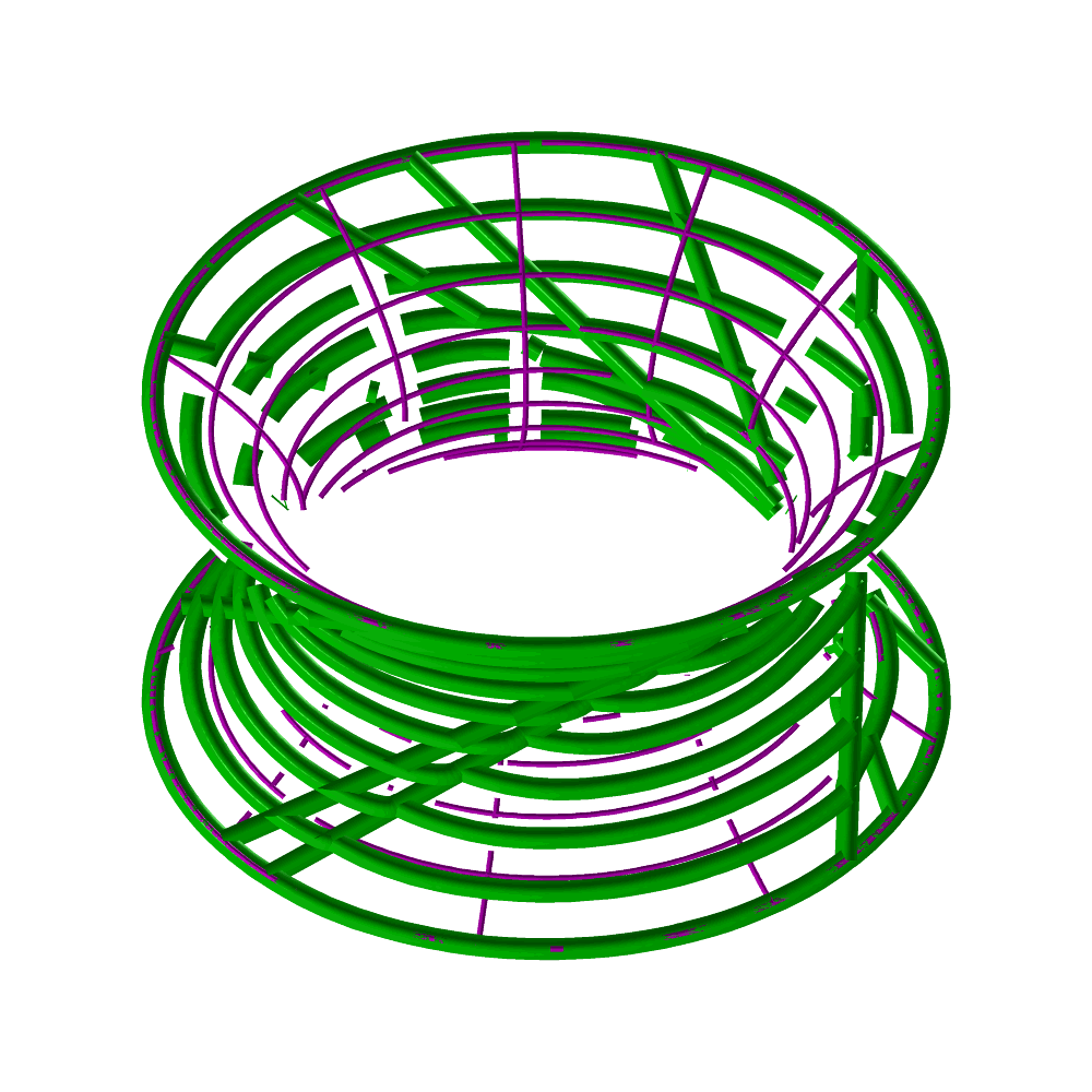
FIGURE:
A ruled surface fitting to a general hyperbolic surface using RULEDFIT.
See also RULEDSRF.
RULEDSRF
SurfaceType RULEDSRF( Mode, CurveType Crv1, CurveType Crv2 )
or
PolygonType RULEDSRF( Mode, PolygonType Poly1, PolygonType Poly2 )
The Mode parameter indicates which variant of the operator
to use. For regular ruling operator, it should be 0. The regular
operator construct a ruled surface between the two curves Crv1
and Crv2 or two polylines Poly1 and Poly2. If The
curves do not have to have the same order or type, and will be
promoted to their least common denominator. The polys must have the
same number of points and both must be either polygons or polylines.
For a Kernel-based ruling operator, which is used to construct valid
planar ruled surface (aiming to ensure positive Jacobian throughout
the domain, while parametrization will no longer will be linear
between the input curves), the Mode parameter should be a list
of five numeric values:
( Op, DistRatio, Limit, SubEps, IsSingular), where
Op is either 0 or 1 for adding DOFs using degree raising or knot
insertion, respectively.
DistRatio is a number in [0, 1] to set how far to move internal
control points toward the kernel.
If 1 the points are moved to the kernel point.
Place a Limit on the number of knots to add or the maximal
degree in degree raising.
SubEps is the Subdivision epsilon. 0.01 is a reasonable start for
a unit size geometry.
IsSingular can be:
TRUE to allow singularity at the kernel point.
FALSE all the surface is regular.
The Kernel-based ruling operator, if successful, constructs a valid
ruled surface between Crv1 and Crv2, which has the same
boundaries as the regular ruled surface, but its interior
parametrization will be non linear.
Example:
c1 = cbspline( 3,
list( ctlpt(E3, 1.7, 0.0 , 0 ),
ctlpt(E3, 0.7, 0.7 , 0 ),
ctlpt(E3, 1.7, 0.3 , 0 ),
ctlpt(E3, 1.5, 0.8 , 0 ),
ctlpt(E3, 1.6, 1.0 , 0 ) ),
list( KV_OPEN ) );
c2 = cbspline( 3,
list( ctlpt(E3, 0.7, 0.0 , 0 ),
ctlpt(E3,-0.7, 0.2 , 0 ),
ctlpt(E3, 0.7, 0.5 , 0 ),
ctlpt(E3,-0.7, 0.7 , 0 ),
ctlpt(E3, 0.7, 1.0 , 0 ) ) ,
list( KV_OPEN ) );
srf1 = RULEDSRF( 0, c1, c2 );
interact( list( c1, c2, srf1 ), on );
c2a = ffmatch( c1, c2, 50, 100, 2, false, 1 );
srf2 = RULEDSRF( 0, c1, c2a );
interact( list( c1, c2, srf2 ), on );
constructs a planar ruled surface between two curves, c1 and c2.
The naive construction causes self intersection, but by employing FFMATCH
the self intersection can be resolved.
See figure for an example.
c1 = cbezier(
list( ctlpt( E2, -1., -1. ),
ctlpt( E2, -0.724, -1.973 ),
ctlpt( E2, 1.026, -1.983 ),
ctlpt( E2, -0.756, -0.283 ),
ctlpt( E2, 1., -1. ) ) );
c2 = cbezier(
list( ctlpt( E2, -1., 1. ),
ctlpt( E2, -0.738, 0.975 ),
ctlpt( E2, -1.639, 1.54 ),
ctlpt( E2, -1.965, 1.636 ),
ctlpt( E2, 1., 1. ) ) );
srf1 = RULEDSRF( 0, c1, c2 );
interact( list( c1, c2, srf1 ), on );
srf2 = RULEDSRF( list( 0, 1.0, 5, 0.01, TRUE ), bottom , top ) * tx(-3);
srf3 = RULEDSRF( list( 1, 1.0, 5, 0.01, TRUE ), bottom, top ) * tx(3);
interact( list( c1, c2, srf1, srf2, srf3 ), on );
constructs a planar ruled surface between two curves, c1 and c2.
The naive construction causes self intersection. By using the kernel-based
ruling operator, the self intersection can be resolved. After adding degree
of freedoms to the input curves using either degree raising operator or
refinement.
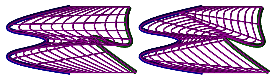
FIGURE:
A naive construction of a ruled surface (left) using RULEDSRF
results in self intersection. FFMATCH is employed (right) to
automatically resolve this self intersection.
See also SRFORTHONET, RULEDTV, RULEDVMDL, FFMATCH and RULEDFIT.
RULEDTV
TrivarType RULEDTV( Mode, SurfaceType Srf1, SurfaceType Srf2 )
Mode parameter indicates which variant of the operator to use.
For regular ruling operator, should be 0. The regular operator
constructs a ruled trivariate between the two surfaces Srf1 and
Srf2.
The surfaces do not have to have the same order or type, and will be
promoted to their least common denominator.
For a Kernel-based ruling operator, which is used to construct valid
trivariate (i.e. with positive Jacobian throughout the domain, if possible),
the Mode parameter should be a list of five numeric values:
( Op, DistRatio, Limit, SubEps, IsSingular), where
Op is either 0 or 1 for adding DOFs using degree raising or knot
insertion, respectively.
DistRatio is a number in [0, 1] to set how far to move internal
control points toward the kernel.
If 1 the points are moved to the kernel point.
Place a Limit on the number of knots to add or the maximal
degree in degree raising.
SubEps is the Subdivision epsilon. 0.01 is a reasonable start for
a unit size geometry.
IsSingular can be:
TRUE to allow singularity at the kernel point.
FALSE all the surface is regular.
The Kernel-based ruling operator, if successful, constructs a valid ruled
trivariate between Srf1 and Srf2, which has the same boundaries
as the regular ruled trivariate, but its interior parametrization will be
non linear.
Example:
s1 = boolone( pcircle( vector( 0, 0, 0 ), 1 ) );
s2 = boolone( pcircle( vector( 0, 0, 1 ), 0.5 ) );
tv = RULEDTV( 0, s1, s2 );
constructs a truncated cone-volume as a ruled trivariate between two surfaces,
s1 and s2.
See figure for an example.
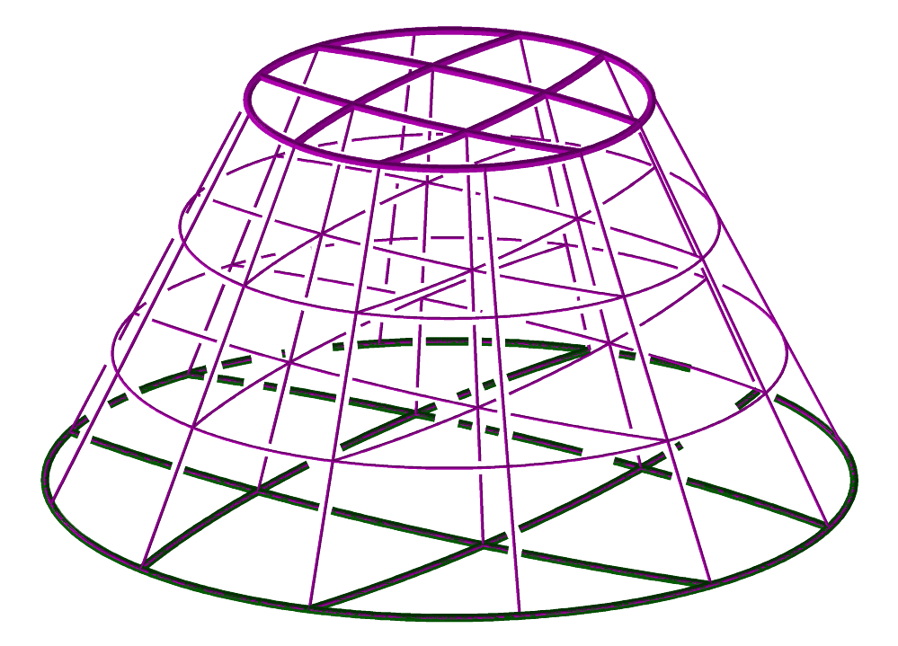
FIGURE:
A ruled volume as a trivariate between two disc surfaces, created via
the RULEDTV function.
See also RULEDSRF, RULEDVMDL, EXTRUDE, and TFROMSRFS.
RULEDVMDL
TrivarType RULEDVMDL( TrimSrfType TSrf1, SurfaceType Srf2, NumericType ResultType )
Constructs a ruled volumetric model (as a trimmed trivariate) between the
two surfaces TSrf1 and Srf2.
The trimming curves of TSrf1 will be extruded into the third dimension
of the volume and will be employed as the trimming surfaces of the result.
The result will be a VModelType if ResultType is TRUE and a ModelType
otherwise.
The surfaces do not have to have the same order or type, and will be
promoted to their least common denominator.
Example:
RuledVModel = RULEDVMDL( tsrf, s * sc( 0.9 ), true );
See also VMDLSWP, VMDLREV, RULEDSRF, EXTRUDE, and TFROMSRFS.
SACCESS
ListType SACCESS( SurfaceType AccessSrf,
AnyType OrientFieldSrf,
SurfaceType CheckSrf,
NumericType SubdivTol,
NumericType NumericTol )
computes the domain on the AccessSrf surface that is accessible from the
orientation that is optionally prescribed by OrientFieldSrf, without
gouging into the CheckSrf surface. If OrientFieldSrf is not
a surface, the normal field of AccessSrf is employed.
AccessSrf and OrientFieldSrf must share a (u, v) domain,
whereas CheckSrf can present a different (s, t) domain.
The accuracy of the computation is governed by a two stage solution,
a subdivision stage with tolerance SubdivTol followed by a numerical
improvement stage with NumericTol accuracy. The second, numeric,
stage is invoked only if NumericTol < SubdivTol.
The returned results are a set of points on the boundary of the accessible
region. The points are in E4 space as (u, v, s, t) 4-tuples.
Example:
c = cregion( pcircle( vector( 0, 0, 0 ), 1 ), 1, 3 ) * ry( 90 );
pSphere = surfPRev( c ) * sc( 0.3 ) * tz( 1 );
Pln = ruledSrf( 0,
ctlpt( E3, -1, -1, 0 ) + ctlpt( E3, -1, 1, 0 ),
ctlpt( E3, 1, -1, 0 ) + ctlpt( E3, 1, 1, 0 ) );
Pts = SACCESS( Pln, 0, pSphere, 0.1, 1e-5 );
sPts = nil();
sPtsErr = nil();
for ( i = 1, 1, sizeof( Pts ),
Pt = nth( Pts, i ):
Err = getAttr( Pt, "Error"):
if ( Err > 1e-5,
snoc( seval( Pln, coord( Pt, 1 ), coord( Pt, 2 ) ), sPtsErr ),
snoc( seval( Pln, coord( Pt, 1 ), coord( Pt, 2 ) ), sPts ) ) );
color( sPts, green );
color( sPtsErr, red );
interact( list( pSphere, Pln, sPts, sPtsErr ) );
computes the access domain of plane Pln along the normal, Z, direction
while preventing gouging into the check surface pSphere.
See figure for an example.
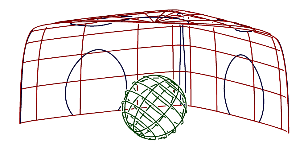
FIGURE:
The limit of the accessible area of the plane along the normal
direction, without gouging into the sphere is computed and presented
using the SACCESS function.
See MZERO for the meaning of SubdivTol and NumerTol.
SADAPISO
CurveType SADAPISO( SurfaceType Srf, NumericType OutputType, NumericType Dir,
NumericType Eps, NumericType FullIso,
NumericType SinglePath, ListType WeightPtSclWdt )
Constructs a coverage to Srf using isocurves, if
OutputType is 1, in the Dir direction and simple iso-distance
function. If OutputType is 2, the used iso-distance function takes
into account the skewing in the transformation (i.e. the
non-orthogonality on conformality). Finally, if OutputType is
0, the constructed coverage to Srf will be using
quadrilaterals.
The coverage to the surface Srf is in the following sense,
using isocuves, for any point p on surface Srf, there exists a
point on one of the isocurves that is close to p within Eps.
If FullIso, the extracted isocurves span the entire surface domain;
otherwise they may span only a subset of the domain. If SinglePath,
an approximation to a single path (Hamiltonian path) that visits all
isocurves is constructed (not supported).
If Srf has an integer "AdapIsoMinSubdivLevel" attribute, it is used
to set the minimal subdivision level used in the adaptive isocurve
computations.
If quadrilaterals are generated, one can force higher density of quads at
some zone using the WeightPtSclWdt parameter that is a list of length
three: (point of interest, weight of influence, scale factor).
See also COVERPT, COVERISO.
srf = sbezier( list( list( ctlpt( E3, -0.5, -1.0, 0.0 ),
ctlpt( E3, 0.4, 0.0, 0.1 ),
ctlpt( E3, -0.5, 1.0, 0.0 ) ),
list( ctlpt( E3, 0.0, -0.7, 0.1 ),
ctlpt( E3, 0.0, 0.0, 0.0 ),
ctlpt( E3, 0.0, 0.7, -0.2 ) ),
list( ctlpt( E3, 0.5, -1.0, 0.1 ),
ctlpt( E3, -0.4, 0.0, 0.0 ),
ctlpt( E3, 0.5, 1.0, -0.2 ) ) ) );
attrib( srf, "AdapIsoMinSubdivLevel", 2 );
aiso = SADAPISO( srf, TRUE, COL, 0.1, FALSE, FALSE, NIL() );
constructs an adaptive isocurve approximation with tolerance of 0.1 to
surface srf in direction COL. Isocurves are allowed to span a
subset of the surface domain. No single path is needed.
The SinglePath option is currently not supported. See also TADAPISO.
SASPCTGRPH
PolyType SASPCTGRPH( SurfaceType Srf )
approximates the aspect graph of surface Srf by computing the
principal directions with zero curvature at the parabolic points of Srf.
The aspect graph is defined over the unit sphere and identifies all
direction from which the silhouette curves of Srf change topology.
Example:
AG = SAspctGrph( Srf );
See also SILHOUETTE.
SASYMPEVAL
ListType SASYMPEVAL( SurfaceType Srf, NumericType U, NumericType V,
NumericType Euclidean )
evalutes the asymptotic direction of surface Srf at parametric
location (U, V), if any. If Euclidean is not zero, the directions
are returned in Euclidean space, otherwise, in parametric space. Returned
is a list of upto two vectors.
Example:
AsympDir = SAsympEval( Srf, u, v, true );
See also SCRVTR.
SBEZIER
SurfaceType SBEZIER( ListType CtlMesh )
creates a Bezier surface using the provided control mesh. CtlMesh is a
list of rows, each of which is a list of control points. All control points
must be of type (E1-E9, P1-P9), or regular PointType defining the surface's
control mesh. The surface's point type will be of a space which is the
union of the spaces of all points.
Example:
Srf = SBEZIER( list ( list( ctlpt( E3, 0.0, 0.0, 1.0 ),
ctlpt( E3, 0.0, 1.0, 0.0 ),
ctlpt( E3, 0.0, 2.0, 1.0 ) ),
list( ctlpt( E3, 1.0, 0.0, 0.0 ),
ctlpt( E3, 1.0, 1.0, 2.0 ),
ctlpt( E3, 1.0, 2.0, 0.0 ) ),
list( ctlpt( E3, 2.0, 0.0, 2.0 ),
ctlpt( E3, 2.0, 1.0, 0.0 ),
ctlpt( E3, 2.0, 2.0, 2.0 ) ),
list( ctlpt( E3, 3.0, 0.0, 0.0 ),
ctlpt( E3, 3.0, 1.0, 2.0 ),
ctlpt( E3, 3.0, 2.0, 0.0 ) ),
list( ctlpt( E3, 4.0, 0.0, 1.0 ),
ctlpt( E3, 4.0, 1.0, 0.0 ),
ctlpt( E3, 4.0, 2.0, 1.0 ) ) ) );
See figure for an example.
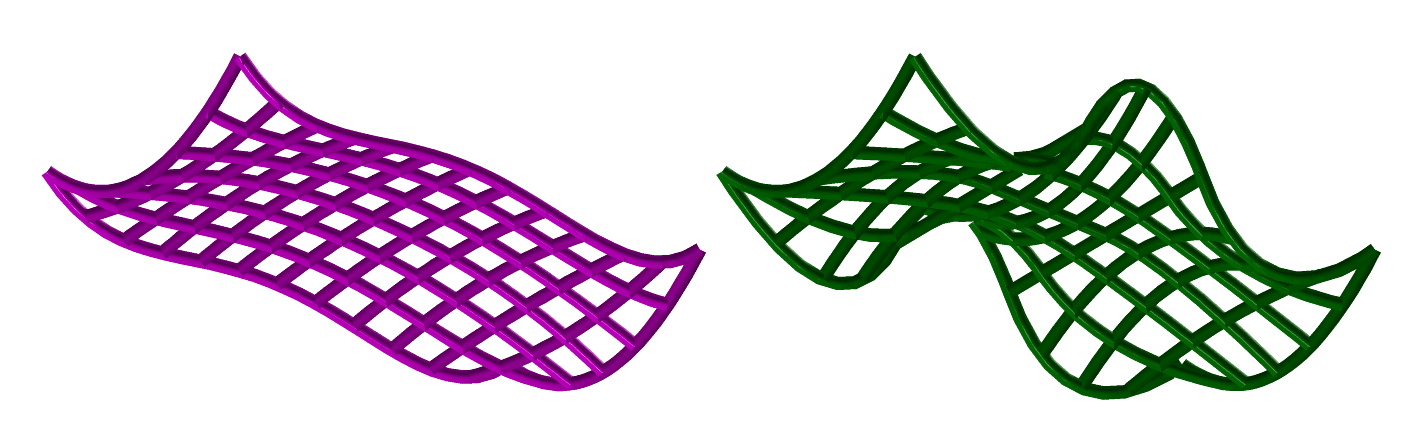
FIGURE:
A Bezier surface (left) of degree 3 by 5 and a B-spline surface (right)
of degree 3 by 3 (bi-quadratic). Both share the same control mesh.
See also CBEZIER, SBSPLINE and SPOWER.
SBISECTOR
SurfaceType SBISECTOR( SurfaceType Srf, PointType Pt )
computes the bisector surface of a given surface to a point.
See also CBISECTOR2D, CBISECTOR3D.
Example:
s = ruledSrf( 0,
ctlpt( E3, -1.0, -1.0, 0.0 ) + ctlpt( E3, 1.0, -1.0, 0.0 ),
ctlpt( E3, -1.0, 1.0, 0.0 ) + ctlpt( E3, 1.0, 1.0, 0.0 ) );
pt = point( 0.0, 0.0, 1.0 );
bisect = SBISECTOR( s, pt );
interact( list( s, pt, bisect ) );
computes the bisector surface of a plane and a point.
See figure for an example.
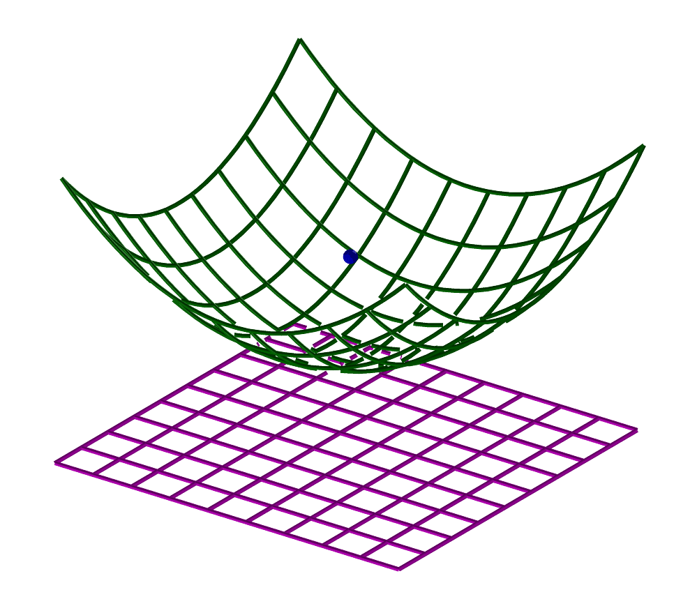
FIGURE:
(a) Bisector surface of a plane and a point computed using the
SBISECTOR command.
SBSPLINE
SurfaceType SBSPLINE( NumericType UOrder, NumericType VOrder,
ListType CtlMesh, ListType KnotVectors )
creates a B-spline surface from the provided UOrder and VOrder
orders, the control mesh CtlMesh, and the two knot vectors KnotVectors.
CtlMesh is a list of rows, each of which is a list of control points.
All control points must be of point type (E1-E9, P1-P9), or regular
PointType defining the surface's control mesh. The surface's point type will
be of a space which is the union of the spaces of all points.
KnotVectors is a list of two knot vectors. Each knot vector is a
list of NumericType knots of length #CtlPtList plus the Order.
If, however, the length of the knot vector is equal to #CtlPtList +
Order + Order - 1}, the curve is assumed to be periodic.
The knot vector may also be a list of a single constant KV_OPEN or
KV_FLOAT or KV_PERIODIC, in which a uniform knot vector with the
appropriate length and with an open, floating or periodic end condition
will be constructed automatically.
Example:
Mesh = list ( list( ctlpt( E3, 0.0, 0.0, 1.0 ),
ctlpt( E3, 0.0, 1.0, 0.0 ),
ctlpt( E3, 0.0, 2.0, 1.0 ) ),
list( ctlpt( E3, 1.0, 0.0, 0.0 ),
ctlpt( E3, 1.0, 1.0, 2.0 ),
ctlpt( E3, 1.0, 2.0, 0.0 ) ),
list( ctlpt( E3, 2.0, 0.0, 2.0 ),
ctlpt( E3, 2.0, 1.0, 0.0 ),
ctlpt( E3, 2.0, 2.0, 2.0 ) ),
list( ctlpt( E3, 3.0, 0.0, 0.0 ),
ctlpt( E3, 3.0, 1.0, 2.0 ),
ctlpt( E3, 3.0, 2.0, 0.0 ) ),
list( ctlpt( E3, 4.0, 0.0, 1.0 ),
ctlpt( E3, 4.0, 1.0, 0.0 ),
ctlpt( E3, 4.0, 2.0, 1.0 ) ) );
Srf = SBSPLINE( 3, 3, Mesh, list( list( KV_OPEN ),
list( 3, 3, 3, 4, 5, 6, 6, 6 ) ) );
constructs a bi-quadratic B-spline surface with its first knot vector
having a uniform knot spacing with open end conditions.
See figure for an example.
See also CBSPLINE, SBEZIER and SPOWER.
SCINTER
ListType SCINTER( SurfaceType Srf, CurveType Crv,
NumericType SubdivTol, NumericType NumericTol,
NumeircType Euclidean )
Returns the intersection points of Srf S(u, v) and Crv C(t)
in the parametric space if Euclidean FALSE, and in the Euclidean space
if Euclidean TRUE. Parametric locations are returned as (t, u, v)
tuples and Euclidean points as (x, y, z).
SubdivTol and NumericTol sets the accuracy of the computation.
Example:
InterPt = SCINTER( glass, 3DCrv, 0.01, 1e-10, true );
Computes the intersection locations of surface glass and curve 3DCrv,
in Euclidewan space.
See also SLINTER, SSINTER, RRINTER, SSINTR2 and GGINTER.
SCRVTR
SurfaceType SCRVTR( SurfaceType Srf, ConstType PtType, ConstType Dir )
symbolically computes the extreme curvature bound on Srf.
If Dir is either ROW or COL, then the normal curvature square
of Srf in Dir is computed symbolically and returned.
Otherwise, an upper bound on the sum of the squares of the two
principle curvatures is symbolically computed and returned.
The returned value is a surface that can be evaluated to the curvature
bound, given a UV location. The returned surface value is a scalar field
of point type P1 (scalar rational).
However, if PtType is one of E1, P1, E3, or P3, the returned surface
is coerced to this given type. If the types are one of E3, or P3, then the
Y and Z axes are set to be equivalent to the U and V parametric domains.
This function computes the square of the normal curvature scalar
field for surfaces as (in the U parametric direction, same for V),
2
d S
< n , --- >
2
u du
k (u, v) = ------------
n
dS ds
< -- , -- >
du du
and computes the sum of the squares of the principle curvatures as,
2 2 ( g11 l22 + g22 l11 - 2 g12 l12 )^2 - 2 |G| |L|
k + k = -----------------------------------------------
1 2 |G|^2 ||n||^2
See also CCRVTR, SCRVTREVAL, SASYMPEVAL.
Example:
cross = cbspline( 3,
list( ctlpt( E2, 0.0, 0.0 ),
ctlpt( E2, 0.8, 0.0 ),
ctlpt( E2, 0.8, 0.2 ),
ctlpt( E2, 0.07, 1.4 ),
ctlpt( E2, -0.07, 1.4 ),
ctlpt( E2, -0.8, 0.2 ),
ctlpt( E2, -0.8, 0.0 ),
ctlpt( E2, 0.0, 0.0 ) ),
list( KV_OPEN ) );
cross = coerce( cross, e3 );
s = sFromCrvs( list( cross,
cross * trans( vector( 0.5, 0, 1 ) ),
cross * trans( vector( 0, 0, 2 ) ) ), 3, KV_OPEN );
view( list( s, axes ), on );
UCrvtrZXY = scrvtr( s, E3, row );
VCrvtrZXY = scrvtr( s, E3, col );
UCrvtrXYZ = UCrvtrZXY * rotx( -90 ) * roty( -90 ) * scale( vector( 1, 1, 0.001 ) );
VCrvtrXYZ = VCrvtrZXY * rotx( -90 ) * roty( -90 ) * scale( vector( 1, 1, 10 ) );
color( UCrvtrXYZ, red );
color( VCrvtrXYZ, magenta );
view( list( UCrvtrXYZ, VCrvtrXYZ ), off );
CrvtrZXY = scrvtr( s, E3, off );
CrvtrXYZ = CrvtrZXY * rotx( -90 ) * roty( -90 ) * scale( vector( 1, 1, 0.001 ) );
color( CrvtrXYZ, green );
view( CrvtrXYZ, off );
computes the square of the normal curvature in the U and V directions, flips
its scalar value from X to Z using rotations and scales the fields to
reasonable values, and then displays them.
It also displays a total bound on the normal curvature.
Due to the large degree of the resulting fields, be aware that rational
surfaces will compute into large degree curvature bound fields. See also
IRITSTATE "InterpProd" option for faster symbolic computation.
See figure for an example.
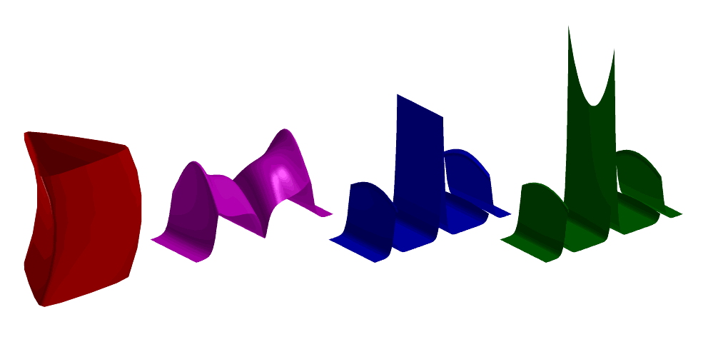
FIGURE:
From left to right: original surface, normal curvature in the U
direction, normal curvature in the V direction, sum of the square of
principle curvatures (different scales).
All computed using SCRVTR.
SCRVTREVAL
ListType SCRVTREVAL( SurfaceType Srf, NumericType U, NumericType V,
NumericType Euclidean )
computes the principle curvatures and directions of surface Srf
at parametric location (U, V). A list of four elements
(k1, V1, k2, V2), with k1/V1 being the first principle curvature/direction
and k2/V2 being the second, is returned. If Euclidean is TRUE then
the principle curvatures are returned in Euclidean space.
Consecutive calls with the same surface Srf to SCRVTREVAL will yield
more efficient evaluations as derivative data is cached.
Example:
Crvtr = SCRVTREVAL( Srf, 0.5, 0.5, True );
K = nth( Crvtr, 1 ) * nth( Crvtr, 3 );
computes the Total (Gaussian) curvatures, K = k1 * k2, of Srf at (0.5, 0.5).
See also SCRVTR.
SDDMMAP
PolyType SDDMMAP( SurfaceType BaseSrf, PolyType Bump,
NumericType UDup, NumericTye VDup, NumericTye LclUVs )
Tiles a composition of Bump over surface BaseSrf
UDup by VDup times, creating a detailed bump geometry. Bump
can be any polygonal geometry whatsoever with XY coordinates that are
contained in the unit square [0, 1] x [0, 1], while Z serves as the elevation
above the surface. The composed geometry could inherit the UV texture
ccordinates from the UV coordinates found in Bump if LclUVs is TRUE
or inherit BaseSrf UV coordinates if LclUVs is FALSE.
Example:
BaseTorus = torusSrf( 1, 0.2 );
BumpTorus = SDDMMAP( BaseTorus, BumpPolyObj, 6, 8, on );
constructs a bumpy BumpTorus with a bump tiled 6 x 8 times over the
surface.
See figure for an example.
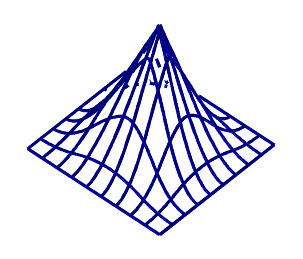 +
+
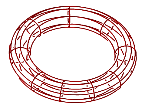 =
=
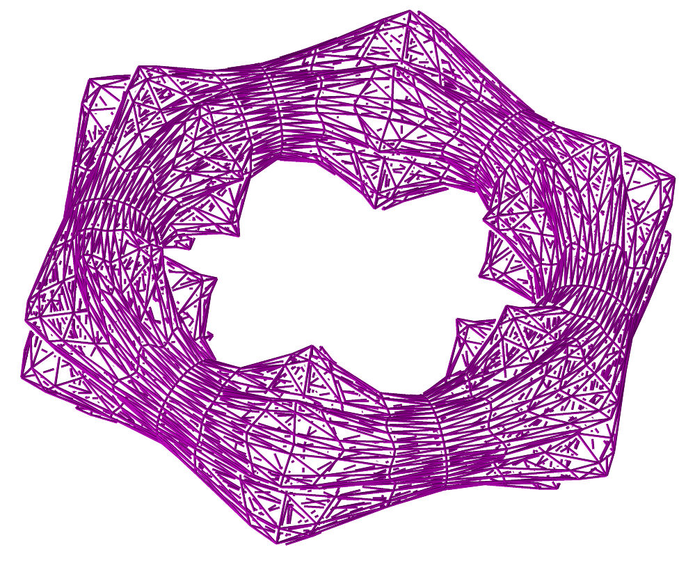
FIGURE:
Polygonal geometry (left) could be tiled over arbitrary surface,
torus in this case (middle), to yield a bumpy shape (right)
using the SDDMMAP function.
See also TEXTWARP, TDEFORM.
SDERIVE
SurfaceType SDERIVE( SurfaceType Srf, NumericType Dir )
returns a vector field surface representing the differentiated surface
in the given direction (ROW or COL). Evaluation of the returned surface at
a given parameter value will return a vector tangent to Srf in
Dir at that parameter value.
DuSrf = SDERIVE( Srf, ROW );
DvSrf = SDERIVE( Srf, COL );
Normal = coerce( seval( DuSrf, 0.5, 0.5 ), VECTOR_TYPE ) ^
coerce( seval( DvSrf, 0.5, 0.5 ), VECTOR_TYPE );
computes the two partial derivatives of the surface Srf and computes
its normal as their cross product, at the parametric location (0.5, 0.5).
See also CDERIVE, TDERIVE, and MDERIVE.
SDIVCRV
CurveType SDIVCRV( SurfaceType Srf, CurveType Crv)
subdivides surface Srf into two along curve Crv, assuming that:
Crv is a simple curve in the UV parametrci domain of Srf and
that Crv divides the domain of Srf into two regions by starting
and ending on two opposite boundaries of Srf. Either Crv starts
and ends in UMin/UMax or VMin/VMax of Srf.
Example:
Srfs = SDIVCRV( Srf, Crv );
See figure for an example.
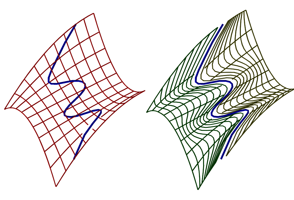
FIGURE:
A surface can be subdivided along a general curve that splits its domain
into two distinct regions using SDIVCRV. Left shows the input and the
right shows the result (after shifting a bit the two surface regions).
See also SDIVIDE.
SDIVIDE
SurfaceType SDIVIDE( SurfaceType Srf, ConstantType Direction,
NumericType Param )
or
TrimSrfType SDIVIDE( TrimSrfType Srf, ConstantType Direction,
NumericType Param )
subdivide a (possibly trimmed) surface into two at the specified parameter
value Param in the specified Direction (ROW or COL). Srf
can be either a B-spline surface in which Param must be contained in
the parametric domain of the surface, or a Bezier surface in which Param} can be arbitrary, extrapolating if not in the range of zero to one.
It returns a list of upto two sub-surfaces. The individual surfaces may be
extracted from the list using the NTH command. If Srf is a trimmed
surface, it may be the case that one of the two subdivided surfaces is
completely trimmed out, and hence only one surface will be returned.
Example:
SrfLst = SDIVIDE( Srf, ROW, 0.5 );
Srf1 = nth( SrfLst, 1 );
Srf2 = nth( SrfLst, 2 );
subdivides Srf at the parameter value of 0.5 in the ROW direction.
See figure for an example.
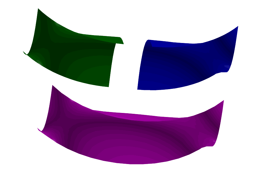
FIGURE:
A surface can be subdivided into two distinct regions using SDIVIDE.
See also CDIVIDE, SDIVCRV, TDIVIDE, and MDIVIDE
SDVLPCRV
SurfaceType SDVLPCRV( SurfaceType Srf, CurveType Crv, ListType Params )
constructs a developable surface, give curve Crv and surface Srf.
If Crv is a 2D curve, it is assumed in the parametric domain of
Srf and a developable sheet that is tangent to Srf along Crv
is constructed. In this case, Params holds only one NumericType
parameter setting the scaling of the constructed developable surface in the
ruling direction.
If Crv is a 3D curve, a developable sheet is constructed that is
in tangential contant with both curve Crv and surface Srf. Then,
Params is a list of five parameteras as
(OrientField, SubdivTol, NumericTol, Euclidean, CrvReduction) where
OrientField, if is a curve, prescribes where to look for solutions of the
next developable in the surface (u, v) space, along Crv params. This
optional curve is assumed to have the same parameterization as Crv.
SubdivTol, NumericTol: Controls the solution process tolerances and
Euclidean is TRUE to return the construct developable scroll(s) in the
Euclidean space, or otherwise it will be returned in (u, v, t) space.
Finally, CrvSizeReduction allows a reduction in size of traced curve
while ensuring the Tolerance, conservatively.
Example:
DvlpSrf = SDVLPCRV( Srf, Circ, list( 0.03 ) );
constructs a developable surface that is tangent to Srf along
Circ that is the parametric domain of Srf.
See also PRISA, DVLPSTRIP and PRULEDALG
SELFINTER
ListType SELFINTER( CurveType Crv, NumericType SubdivTol,
NumericType NumerTol, NumericType MinNrmlDeviation,
NumericType Euclidean )
or
ListType SELFINTER( SurfaceType Srf, NumericType SubdivTol,
NumericType NumerTol, NumericType MinNrmlDeviation,
NumericType Euclidean )
computes the self intersection locations/curves of a given curve or
surface. Returned is a list of points/piecewise linear curves. The
returned locations, if in the parameteric space (see below), are pairs
of parameter values along the curve in case of a curve and a 4-tuple
holding the pair of surface location, in case of surfaces.
See MZERO for the meaning of SubdivTol and NumerTol.
If MinNrmlDeviation is positive it specifies the minimal deviation
angle required for the two normal at the self intersection (of the two
different interesecting locations), in degrees. If -1, a different
approach algother is used that eliminates the redundant diagonal factor
in the self intersection constraint. If -2, miter (singular Jacobian)
locations are computed.
If Euclidean, the returned data is in Euclidean space. Otherwise,
the returned data is in parameteric space.
Example:
si1 = selfinter( crv, 0.001, 1e-10, 15.0, true );
si2 = selfinter( crv, 0.001, 1e-10, -1.0, true );
See also PSELFINTER
SETCOVER
ListType SETCOVER( ListType RangesSet, NumericType OverlapTolerance )
computes the minimal subset of the given set RangesSet, that covers
the entire domain spanned by RangesSet. A range is a list object with
two numeric values, the start and end of this specific range. Each element
in RangesSet can be either a range, or a list of ranges.
OverlapTolerance specifies the tolerance to use in overlapping
ranges.
Returned is a list of indices (first element zero) that prescribe the
minimal coverage.
Note that the former case of a single range per element is solved in an
almost linear time whereas the later case of multiple ranges per element is
exponential. Hence, do not attempt to find minimal coverage of more than a
few elements in the later case.
Example:
Ranges = list( list( 0.0, 0.4 ),
list( 0.1, 0.4 ),
list( 0.3, 1.0 ),
list( 0.1, 0.9 ) );
Indcs = SETCOVER( Ranges, 1e-7 );
and SETCOVER should return "list( 0, 2 )", the two indices of the ranges
that cover this domain of [0, 1]. See also CVISIBLE.
SEDITPT
SurfaceType SEDITPT( SurfaceType Srf, CtlPtType CPt, NumericType UIndex,
NumericType VIndex )
provides a simple mechanism to manually modify a single control point number
UIndex and VIndex (base count is 0) in the control mesh of Srf
by substituting CtlPt instead. CtlPt must have the same point type as
the control points of Srf. The original surface Srf is not modified.
Example:
CPt = ctlpt( E3, 1, 2, 3 );
NewSrf = SEDITPT( Srf, CPt, 0, 0 );
constructs a NewSrf with the first control point of Srf being
CPt.
SEVAL
CtlPtType SEVAL( SurfaceType Srf, NumericType UParam, NumericType VParam )
or
CtlPtType SEVAL( TrimSrfType Srf, NumericType UParam, NumericType VParam )
evaluates the provided (possibly trimmed) surface Srf at the given
UParam and VParam parameters. Both UParam and VParam
should be contained in the surface parametric domain if Srf is a
B-spline surface, or between zero and one if Srf is a Bezier surface.
The returned control point has the same type as the control points of
Srf.
Example:
CPt = SEVAL( Srf, 0.25, 0.22 );
evaluates Srf at the parameter values of (0.25, 0.22).
See also CEVAL, MEVAL, TEVAL.
SFLECNODAL
PolyType SFLECNODAL( SurfaceType Srf, NumericType SubdivTol,
NumericType NumericTol, NumericType ContactOrder )
computes the flecnodal curves over a given freeform geometry, Srf,
if ContactOrder is 4..
The flecnodal curves are curves of contact of order three with a line in
an asymptotic direction. SubdivTol and NumericTol controls the
subdivision and numeric tolerances of the approximation. Typically the
subdivision tolerance is fairly coarse.
This function can also be used to compute flecnodal points of contact,
if ContactOrder is set to 4.
Example:
flecs = SFlecnodal( srf, 0.05, -1e-6, 3 );
See also MZERO for the meaning of SubdivTol and NumerTol.
SFOCAL
SurfaceType SFOCAL( SurfaceType Srf, NumericType Dir )
evaluates the focal surface field of surface Srf using the normal
curvature in the isoparametric direction as given by Dir (either
ROW or COL). Note this function is not using the principal curvatures as
is generaly the case for focal surfaces.
Example:
gcross = cbspline( 3,
list( ctlpt( E3, 0.3, 0.0, 0.0 ),
ctlpt( E3, 0.1, 0.0, 0.1 ),
ctlpt( E3, 0.1, 0.0, 0.4 ),
ctlpt( E3, 0.5, 0.0, 0.5 ),
ctlpt( E3, 0.6, 0.0, 0.8 ) ),
list( KV_OPEN ) );
glass = surfprev( gcross );
color( glass, red );
gfocal = SFOCAL(glass, col);
evaluates the focal surface using the COL isoparametric direction's
normal curvature of the glass surface.
See figure for an example.
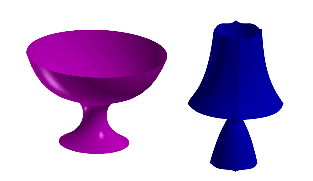
FIGURE:
A focal surface (right) of a glass surface (left) can be computed
using SFOCAL.
SFXCRVTRLN
SurfaceType SFXCRVTRLN( SurfaceType Srf,
NumericType k1,
NumericType Step,
NumericType SubdivTol,
NumericType NumerTol,
NumericType Euclidean )
Comptues the lines of curvatures of surface Srf where one principle
curvature is fixed to the value of k1, if any.
Step, SubdivTol, and NumerTol controls the step size and
tolerances of the approximated curvature lins.
If Euclidean is TURE, the result is returned in Euclidean space.
Otherwise, a parameteric curve will be resulted in Srf.
Example:
CLns5 = sFxCrvtrLn( s, 1, 0.003, 0.001, 1e-8, TRUE );
SFROMCRVS
SurfaceType SFROMCRVS( ListType CrvList,
NumericType OtherOrder,
NumericType OtherEndCond )
or
SurfaceType SFROMCRVS( ListType CrvList,
NumericType OtherOrder,
ListType OtherKnotVector )
constructs a surface by substituting the curves in CrvList as rows
in a control mesh of a surface. The curves in CrvList are made compatible
by promoting Bezier curves to B-splines if necessary, and raising the degrees
and refining as required before substituting the control polygons of the
curves as rows in the mesh. The other direction order is set by
OtherOrder, which cannot be larger than the number of curves.
If B-spline (OtherOrder is smaller than number of curves) end
conditions are set via OtherEndCond and can either be one of
KV_OPEN, KV_FLOAT or KV_PERIODIC, or an explicitly
prescribed knot vector OtherKnotVector.
The surface interpolates the first and last curves only, if a Bezier
or open end conditions are selected; otherwise, no curve is interpolated.
See also SINTERP, SINTPCRVS, TFROMSRFS.
Example:
Crv1 = cbspline( 3,
list( ctlpt( E3, 0.0, 0.0, 0.0 ),
ctlpt( E3, 1.0, 0.0, 0.0 ),
ctlpt( E3, 1.0, 1.0, 0.0 ) ),
list( KV_OPEN ) );
Crv2 = Crv1 * trans( vector( 0.0, 0.0, 1.0 ) );
Crv3 = Crv2 * trans( vector( 0.0, 1.0, 0.0 ) );
Srf = SFROMCRVS( list( Crv1, Crv2, Crv3 ), 3, KV_OPEN );
See figure for an example.

FIGURE:
A surface can be constructed from a list of curves substituted
as rows into its mesh using SFROMCRVS. The surface does not
necessarily interpolate the curves.
SGAUSS
SurfaceType SGAUSS( SurfaceType Srf, NumericType NumerOnly )
evaluates the Gaussian curvature (K) field of surface Srf. If
NumerOnly is TRUE, only the numerator of the Gaussian curvature
is derived. Otherwise, if NumerOnly is FALSE, the full exact
Gaussian field is derived. NumerOnly TRUE may be used in cases
where the zero set of K is needed (parabolic lines).
Example:
Srf1 = hermite( cbezier( list( ctlpt( E3, 0.0, 0.0, 0.0 ),
ctlpt( E3, 0.5, 0.2, 0.0 ),
ctlpt( E3, 1.0, 0.0, 0.0 ) ) ),
cbezier( list( ctlpt( E3, 0.0, 1.0, 0.0 ),
ctlpt( E3, 0.5, 0.8, 0.0 ),
ctlpt( E3, 1.0, 1.0, 0.5 ) ) ),
cbezier( list( ctlpt( E3, 0.0, 2.0, 0.0 ),
ctlpt( E3, 0.0, 2.0, 0.0 ),
ctlpt( E3, 0.0, 2.0, 0.0 ) ) ),
cbezier( list( ctlpt( E3, 0.0, 2.0, 0.0 ),
ctlpt( E3, 0.0, 2.0, 0.0 ),
ctlpt( E3, 0.0, 2.0, 0.0 ) ) ) );
SGauss = SGAUSS( Srf1, false );
evaluates the Gaussian curvaure of Srf1.
See figure for an example.
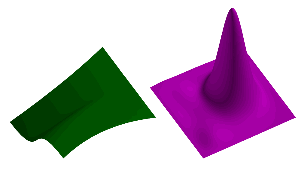
FIGURE:
The Gaussian curvature field (right) of the quadratic by
cubic surface (left) is computed using SGAUSS. The Gaussian
curvature field is scaled down to %1 to fit into the figure.
Compare with figure~protectref{fig-smean}.
See also EVOLUTE and SMEAN.
SILHOUETTE
PolyType SILHOUETTE( SurfaceType Srf, VectorType ViewDir,
NumericType SubdivTol, NumericType Euc )
or
PolyType SILHOUETTE( PolyType Pl, VectorType ViewDir,
NumericType SubdivTol, NumericType Euc )
Compute the silhouette edges of the given Srf or Pl from the
prescribed viewing direction ViewDir. The end result is a piecewise
linear approximation of the exact silhouette, and its accuracy is controlled
via the SubdivTol, in the case of a freeform surface Srf.
If Euc is TRUE, the silhouette curves are returned on the surface,
in Euclidean space. Otherwise, the silhouette curves are returned in the
parametric space of Srf.
Both Euc and the RESOLUTION variables have no affect in the case of
a polygonal model Pl.
Example:
Resolution = 10;
Sils = SILHOUETTE( glass, vector( 1, -2, 1 ), 0.01, true );
computes the silhouette curves of surface glass as viewed from
viewing direction (1, -2, 1), and returns the silhouette curves
in Euclidean space. See also ISOCLINE, PPROPFTCH and SASPCTGRPH.
SINTERP
SurfaceType SINTERP( ListType PtList, ListType Params )
computes a B-spline polynomial surface that interpolates or approximates
the rectangular grid or scattered set of points in PtList. Two main
options:
1. Params is of the form
list( NumericType UOrder, NumericType VOrder,
NumericType USize, NumericType VSize, ConstantType Param)
2. Params is of the form
list( CrvUMin, CrvUMax, CrvVMin, CrvVMax )
For option 1, the B-spline surface will have orders UOrder and
VOrder and mesh of size USize by VSize control
points. If the PtList data is on a grid (list of lists of the
same size), the knots will be spaced according to Param which
can be one of PARAM_UNIFORM, PARAM_CHORD, PARAM_CENTRIP, or
PARAM_NEILFOL. Currently, only PARAM_UNIFORM is supported. For a
scattered point set, the Param parameter is ignored.
PtList is typically a list of points for grid data in which
all lists carry the same amount of points, thereby defining a
rectangular grid. However, for scattered data interpolation, PtList
can also a linear list of points. All points in PtList must be of
type (E1-E9, P1-P9) control point, or regular PointType.
If USize and VSize are equal to the number of points in
the grid data set of PtList, the resulting surface will
interpolate the data set. Otherwise, if USize or VSize
is less than the number of points in the grid of PtList, the
point data set will be least square approximated. At no time can
USize or VSize be larger that the number of points in
PtList or lower than UOrder and VOrder,
respectively. If USize or VSize are zero, the grid size
is used, forcing an interpolation of the data set.
If PtList contains a linear list of points, these points are
treated as scattered. Each scattered point is assumed to be holding the
parameteric location at which to interpolate its first two coefficients.
The other coefficients are the interpolation values. In other words,
to interpolate scattered data of type E3, E5 control points in a linear
list must be provided in (u, v, x, y, z) format. Scattered data is
interpolated over a unit square (0 to 1) parameteric domain in both u
and v.
For option 2, the four boundary curves are specified and will be used
to force the boundary of the fitted surface to follow. Further, the
orders, sizes and parametrizations will be taken for the fitted surface
from the these four curves.
See also SINTPCRVS, SFROMCRVS, CINTERP.
Example:
pl = nil();
pll = nil();
for ( x = -5, 1, 5,
pl = nil():
for ( y = -5, 1, 5,
snoc( point( x, y, sin( x * Pi / 2 ) * cos( y * Pi / 2 ) ),
pl )
):
snoc( pl, pll ) );
s1 = SINTERP( pll, list( 3, 3, 8, 8, PARAM_UNIFORM ) );
s2 = SINTERP( pll, list( 3, 3, 11, 11, PARAM_UNIFORM ) );
samples an explicit surface sin(x) * cos(y) at a grid of 11 by 11 points,
least square fit with a grid of size of 8 by 8 surface s1, and
interpolates surface s2 using this data set. See also CINTERP and
LINTERP.
See figure for an example.
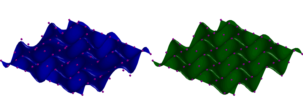
FIGURE:
A surface least square fitting a data set with insufficient
degrees of freedom (left) and actually interpolating the data
set (right), all using SINTERP.
SINTPCRVS
SurfaceType SINTPCRVS( ListType CrvList,
NumericType OtherOrder,
NumericType OtherEndCond,
NumericType OtherParam )
constructs a surface by fitting it to the curves in CrvList. The
curves in CrvList are made compatible by promoting Bezier curves to
B-splines if necessary, and raising the degrees and refining as required
before fitting a surface through them all. The other direction order is
set by OtherOrder, which cannot be larger than the number of curves.
If B-spline (OtherOrder is smaller than number of curves) end
conditions are set via OtherEndCond and can be one of KV_OPEN,
KV_FLOAT or KV_PERIODIC. Finally OtherParam sets the
parametrization in the other direction and can be one of PARAM_CENTRIP,
PARAM_CENTRIP, PARAM_CHORD, or PARAM_NIELFOL.
See also SINTERP, SFROMCRVS.
Example:
Crv1 = cbspline( 3,
list( ctlpt( E3, 0.0, 0.0, 0.0 ),
ctlpt( E3, 1.0, 0.0, 0.0 ),
ctlpt( E3, 1.0, 1.0, 0.0 ) ),
list( KV_OPEN ) );
Crv2 = Crv1 * trans( vector( 0.0, 0.0, 1.0 ) );
Crv3 = Crv2 * trans( vector( 0.0, 1.0, 0.0 ) );
Srf = SINTPCRVS( list( Crv1, Crv2, Crv3 ), 3, KV_OPEN, PARAM_CHORD );
See figure for an example.
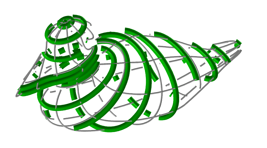
FIGURE:
A surface can be fitted to a list of curves using SINTPCRVS.
SKEL2DINT
ListType SKEL2DINT( CurveType Crv1 | PointType Pt1 | CtlPtType Pt1,
CurveType Crv2 | PointType Pt2 | CtlPtType Pt1,
CurveType Crv3 | PointType Pt3 | CtlPtType Pt1,
NumericType OutExtent, NumericType Epsilon,
NumericType FineNess, ListType MZeroTols )
computes locations in the plane of points that are equadistant from the
three given entities. Entities can be points or control points or curves,
all in the XY plane. The equadistant points are computed as the mutual
intersection of the bisectors of the entities. Infinite bisectors (such
as the bisector of two points) are extended up to OutExtent.
Epsilon controls the tolerances while FineNess controls the
subdivision fineness in the bisector intersection computations.
MZeroTols controls the subdivision/numeric tolerances of the MV solver,
as a list of the two numeric tolerances.
Exanple:
Crv1 = pcircle( vector( -0.5, 0.7, 0.0 ), 0.3 );
Crv2 = pcircle( vector( -0.4, -0.6, 0.0 ), 0.5 );
Crv3 = pcircle( vector( 0.3, 0.2, 0.0 ), 0.4 );
EquaPt = SKEL2DINT( Crv1, Crv2, Crv3, 100, 0.1, 150, list( 1e-3, -1e-9 ) ):
computes the eight points that are equadistant to three circles.
See figure for an example.
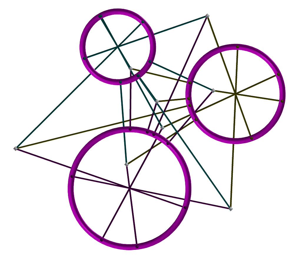
FIGURE:
Computes the eight points that are equadistant to three circles,
using SKEL2DINT.
See also CRC2CRVTAN, TNSCRCR, CRVC1RND, CRV2TANS.
SLINTER
PointType SLINTER( SurfaceType Srf, PointType LinePt, VectorType LineDir,
NumericType SubdivTol, NumericType NumericTol,
NumeircType Euclidean )
Returns the intersection points of Srf S(u, v) and line LinePt
and LineDir as L(t) = LinePos = LineDir t, in the parametric space if
Euclidean FALSE, and in the Euclidean space if Euclidean TRUE.
Parametric locations are returned as
(u, v, 0) tuples and Euclidean points as (x, y, z).
SubdivTol and NumericTol sets the accuracy of the computation.
Example:
InterPt = SLINTER( glass, LinePt, LineDir, 0.01, 1e-10, true );
Computes the intersection locations of surface glass and line
L(t) = LinePos + LineDir t, in Euclidewan space.
Note the line t parameter is not returned and if needed, can be derived
from the Euclidean point solution P as P = L(t) = LinePos + LineDir t.
See also SCINTER, SSINTER, RRINTER, SSINTR2 and GGINTER.
SMEAN
SurfaceType SMEAN( SurfaceType Srf, NumericType NumerOnly )
evaluates the mean curvature field of surface Srf as follows:
if NumerOnly is true, it computes the numerator of only the Mean curvature.
Otherwise, if NumerOnly is false, the square of the exact Mean
curvature field is derived. NumerOnly TRUE may be used in cases
where the zero set of H is needed (k1 == -k2 points).
Example:
Srf1 = hermite( cbezier( list( ctlpt( E3, 0.0, 0.0, 0.0 ),
ctlpt( E3, 0.5, 0.2, 0.0 ),
ctlpt( E3, 1.0, 0.0, 0.0 ) ) ),
cbezier( list( ctlpt( E3, 0.0, 1.0, 0.0 ),
ctlpt( E3, 0.5, 0.8, 0.0 ),
ctlpt( E3, 1.0, 1.0, 0.5 ) ) ),
cbezier( list( ctlpt( E3, 0.0, 2.0, 0.0 ),
ctlpt( E3, 0.0, 2.0, 0.0 ),
ctlpt( E3, 0.0, 2.0, 0.0 ) ) ),
cbezier( list( ctlpt( E3, 0.0, 2.0, 0.0 ),
ctlpt( E3, 0.0, 2.0, 0.0 ),
ctlpt( E3, 0.0, 2.0, 0.0 ) ) ) );
SMean = SMEAN( Srf1, false );
evaluates the square of the mean curvature of Srf1.
See figure for an example.
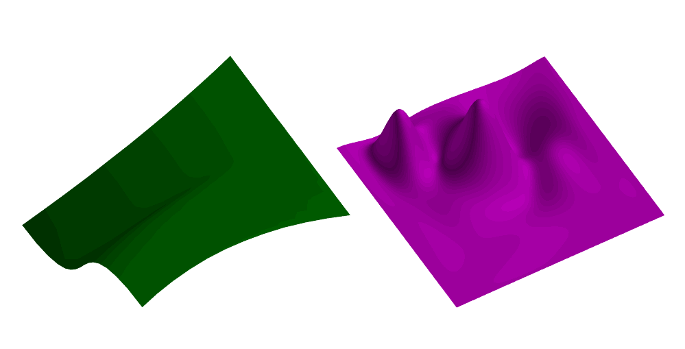
FIGURE:
The square of the mean curvature field (right) of the quadratic by
cubic surface (left) is computed using SMEAN. The square of the
mean curvature field is scaled down to %1 to fit into the figure.
Compare with figure~protectref{fig-sgauss}.
See also EVOLUTE and SGAUSS.
SMERGE
SurfaceType SMERGE( SurfaceType Srf1, SurfaceType Srf2,
NumericType Dir, NumericType SameEdge )
merges two surfaces along the requested direction (ROW or COL). Based on
the value of SameEdge the shared boundary is treated as:
negative The edge is assumed not common and is not interpolated,
leaving a C^-1 discontinuity.
0 The common edge is interpolated (edges are assumed not
identical.
1 The common edge is copied from the 1st surface
2 The common edge is copied from the 2nd surface
3 The common edge is blended between the two surfaces respective
boundaries
Example:
MergedSrf = SMERGE( Srf1, Srf2, ROW, TRUE );
See also MMERGE.
SMESH
SurfaceType SMESH( TrivarType TV, MumericType Dir, NumericType Index )
extracts a surface out of a trivariate, TV, as the Index's plane
of the control mesh of TV in direction Dir. Dir can be
one of COL, ROW, DEPTH.
Example:
tv = tbezier( list( list( list( ctlpt( E3, 0.1, 0.0, 0.8 ),
ctlpt( E3, 0.2, 0.1, 2.4 ) ),
list( ctlpt( E3, 0.3, 2.2, 0.2 ),
ctlpt( E3, 0.4, 2.3, 2.0 ) ) ),
list( list( ctlpt( E3, 2.4, 0.8, 0.1 ),
ctlpt( E3, 2.2, 0.7, 2.3 ) ),
list( ctlpt( E3, 2.3, 2.6, 0.5 ),
ctlpt( E3, 2.1, 2.5, 2.7) ) ) ) );
s0 = SMESH( tv, col, 0 );
s1 = SMESH( tv, col, 1 );
extracts the two (first and last) planes in direction col out of
trivariate tv.
See also STRIVAR, CMESH, MFROMMESH.
SMOEBIUS
CurveType SMOEBIUS( CurveType Crv, NumericType Ratio, NumericType Dir )
rebalances the weights of a rational surface using the Moebius
transformation. The shape of the surface remains identical, while the
speed is modified in the direction Dir.
Ratio controls the ratio between the last and first weights of
the first row/column. If Ratio = 0, the first and last weights are
made equal.
See also CMOEBIUS.
SMOOTHNRML
ListType SMOOTHNRML( ListType Obj, NumericType MaxAngle )
or
PolygonType SMOOTHNRML( PolygonType Obj, NumericType MaxAngle )
Given a (list of) polygonal object(s), Obj, compute normals to
the vertices by averaging the normals of the polygons that share the
vertices. Only vertices where the deviation between the polygons' normals
and the averaged normal is less than MaxAngle are updated. Set to
180 degrees (or more) to enable the blend over all vertices.
If MaxAngle is negative, all vertices normals are cleared and all
polygon normals reevaluated.
This is useful for polygonal data sets that have no vertex normals.
Example:
A = box( vector( -1, -1, -1 ), 2, 2, 2 );
B = SMOOTHNRML( A, 90 );
computes average normals to a curve resulting in the smoothly shaded display
of a cube. See also FIXPLNRML.
SMOMENTS
SurfaceType SMOMENTS( SurfaceType Srf, NumericType Moment,
NumericType Axis1, NumericType Axis2,
NumericType Eval )
or
NumericType SMOMENTS( SurfaceType Srf, NumericType Moment,
NumericType Axis1, NumericType Axis2,
NumericType Eval )
compute the integral moment surface, MSrf, of the given surface
Srf, up to a sign. The computed moment can be either a first order
moment when Moment = 1, or a second order moment when Moment = 2.
If Srf is a closed surface with domain (u0, v0) to (u1, v1), then
the difference of MSrf(u1, v1) - MSrf(u0, v0) is the requested
moment. Otherwise, the computation is for the volume occupied between the
surface Srf and the XY plane.
If Eval is TRUE, the actual numerical value of the moment is returned.
The moment integral surface is returned if Eval is FALSE.
Axis1 and Axis2 prescribe the two axes to compute the moments
for a second order moment computation. For a first order moment
computation only Axis1 is considered.
Example:
Spr = surfPRev( cregion( pcircle( vector( 0, 0, 0 ), 1 ), 1, 3 )
* ry( 90 ) );
SMOMENTS( Spr, 2, 1, 1, 2, 1 );
computes the second order XX moment of a polynomial approximation of a
unit sphere, using method one. See also TVOLUME, SVOLUME, MOMENT and CAREA.
SMORPH
SurfaceType SMORPH( SurfaceType Srf1, SurfaceType Srf2, NumericType Blend )
creates a new surface which is a convex blend of the two given surfaces.
The two given surfaces must be compatible (see FFCOMPAT) before this blend
is invoked. This is very useful if a sequence that "morphs" one surface to
another is to be created.
Example:
for ( i = 0.0, 1.0, 11.0,
Msrf = SMORPH( Srf1, Srf2, i / 11.0 ):
color( Msrf, white ):
attrib( Msrf, "rgb", "255,255,255" ):
attrib( Msrf, "reflect", "0.7" ):
save( "morp1-" + i, Msrf )
);
creates a sequence of 12 surfaces, morphed from Srf1 to Srf2
and saves them in the files "morph-0.itd" to "morph-11.itd".
See also PMORPH, CMORPH and TMORPH.
See figure for an example.
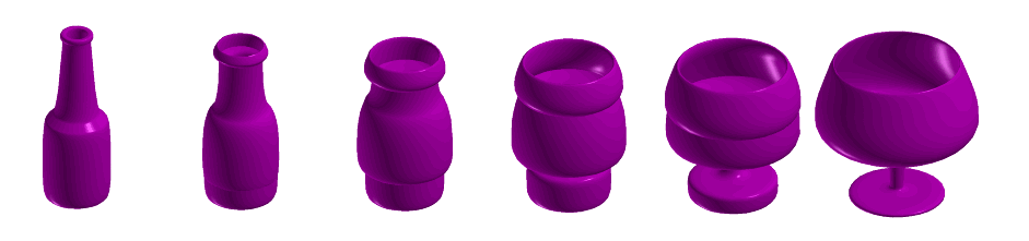
FIGURE:
A morphing sequence between a bottle and a glass. Snapshots computed
using SMORPH.
SNORMAL
VectorType SNORMAL( SurfaceType Srf, NumericType UParam, NumericType VParam )
or
VectorType SNORMAL( TrimSrfType Srf, NumericType UParam, NumericType VParam )
compute the normal vector to (possibly trimmed) surface Srf at the
parameter values UParam and VParam. The returned vector has a
unit length.
Example:
Normal = SNORMAL( Srf, 0.5, 0.5 );
computes the normal to Srf at the parameter values (0.5, 0.5).
See also SNRMLSRF.
SNRMLSRF
SurfaceType SNRMLSRF( SurfaceType Srf )
symbolically computes a vector field surface representing the non-normalized
normals of the given surface. That is, the normal surface, evaluated at
(u, v), provides a vector in the direction of the normal of the original
surface at (u, v). The normal surface is computed as the symbolic cross
product of the two surfaces representing the partial derivatives of the
original surface.
Example:
NrmlSrf = SNRMLSRF( Srf );
See figure for an example.
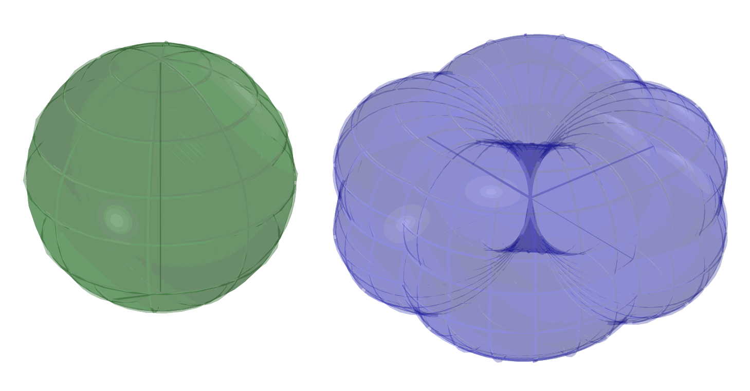
FIGURE:
A vector field normal (right) computed for a unit sphere (left) using
SNRMLSRF. The normal field degenerates at the north and south
poles because the surface is not regular there.
SPARABOLC
ListType SPARABOLC( SurfaceType Srf, NumericType SubdivTol,
NumericType NumericTol, NumericType Euclidean,
DecompSrfs )
computes the parabolic edges of a freeform surface, Srf, as
the zero set of the Gaussian curvature. A scalar field with the sign of
the Gauss curvature is computed and its zero is derived. SubdivTol
and NumericTol controls the subdivision and numeric tolerances of
the approximation. Typically the subdivision tolerance is fairly coarse.
If Euclidean is false, the list of (piecewise linear) parabolic
curves is returned in the parametric space of Srf. Otherwise, if
Euclidean is true, the parabolic curves are mapped onto Srf.
if DecompSrfs is set, the surface is divided into several trimed
surfaces along the parabolic lines, creating regions that are solely
convex, concave, and saddle-like.
Example:
pl = nil();
pll = nil();
for ( x = -3, 1, 3,
pl = nil():
for ( y = -3, 1, 3,
snoc( point( x, y, sin( x * Pi / 2 ) * cos( y * Pi / 2 ) ),
pl ) ):
snoc( pl, pll ) );
EggBase = sinterp( pll, 4, 4, 0, 0, PARAM_UNIFORM );
Resolution = 15;
Parab = SPARABOLC( EggBase, 0.005, 1e-6, true, false );
constructs a surface in the shape of an egg carton's base and then derives its
parabolic edges in Euclidean space.
See also MZERO for the meaning of SubdivTol and NumerTol.
SPHERE
PolygonType SPHERE( VectorType Center, NumericType Radius )
creates a SPHERE geometric object, defined by Center as the center of
the SPHERE, and with Radius as the radius of the SPHERE.
See RESOLUTION for accuracy of SPHERE approximation as a polygonal model.
See IRITSTATE's "PrimRatSrfs" and "PrimRatSrfs" state variables.
SPLITLST
ListType SPLITLST( AnyType LinkedListObj )
splits an object of several linked list data elements such as polygons,
curves, or suraces, into a list object that contains an object for each of
the individual objects.
Example:
ObjLst = SPLITLST( axes );
splits the axes object into a list object of several objects each holding
a single polyline.
See also MERGEPOLY, MERGEPLLN, MERGETYPE, MERGELST.
SPHEREPACK
ListType SPHEREPACK( ModelType Shape, NumericType Radius,
NumericType TimeLimit, BooleanType UseGravity )
Packs a given Shape with spheres in 3D (or circles in 2D) of
a given Radius as densely as possible, within a given TimeLimit,
using either the "Randomize and Repulse" or the "Gravity Shaking" algorithm,
depending on the UseGravity parameter. In 3D, Shape can be
either a closed polygonal model, or a closed C^1 freeform surface. In 2D,
Shape can be either a closed planar polyline or polygon, or a closed
freeform C^1 planar curve.
"Randomize and Repulse" runs in parallel in several threads. "Gravity
Shaking" is single-threaded, but may outperform "Randomize and Repulse"
when thread count is low.
The function returns, in 3D, a list of 7-element tuples, as E7 points,
of the format
(SphereCenterX, SphereCenterY, SphereCenterZ, ClosestBorderPtX,
ClosestBorderPtY, ClosestBorderPtZ, DistToBorderPt).
In 2D, a list of 7-element tuples (E7 Pts) will be returned, of the format
(CircleCenterX, CircleCenterY, 0.0, ClosestBorderPtX, ClosestBorderPtY, 0.0,
DistToBorderPt).
Example:
SpheresInfo = SPHEREPACK( S, 0.06, 60, true );
SPOWER
SurfaceType SPOWER( ListType CtlMesh )
creates a polynomial/rational surface out of the provided control mesh.
The created surface employs the monomial power basis. CtlMesh is a
list of rows, each of which is a list of control points. All control points
must be of type (E1-E9, P1-P9), or regular PointType defining the surface's
control mesh. The surface's point type will be of a space which is the
union of the spaces of all points.
Example:
s = SPOWER( list( list( ctlpt( E3, 1, 0, 1 ),
ctlpt( E3, 0, 1, 1 ) ),
list( ctlpt( E3, 0, 0, 1 ),
ctlpt( E3, 0, 0, 1 ) ) ) );
s == coerce( coerce( s, bezier_type ), power_type );
constructs a bilinear power basis surface, coerces it to a Bezier form,
coerces the Bezier form back to a power basis, and then compares the result
for equality.
See also CBEZIER, SBSPLINE and SPOWER.
SRADCRVTR
SurfaceType SRADCRVTR( SurfaceType Srf, VectorType ViewDir,
NumericType SubdivTol, NumericType SubdivTol,
NUmericType MergeTol )
computes the radial curvature of surface Srf, as viewed from view
direction ViewDir. See MZERO for the meaning of the SubdivTol
and NumerTol tolerances. MergeTol specifies the tolerance to
use to merge points into polygons,
SRAISE
SurfaceType SRAISE( SurfaceType Srf, ConstantType Direction,
NumericType NewOrder )
raises Srf to the specified NewOrder in the specified
Direction.
Example:
Srf = ruledSrf( 0,
cbezier( list( ctlpt( E3, -0.5, -0.5, 0.0 ),
ctlpt( E3, 0.5, -0.5, 0.0 ) ) ),
cbezier( list( ctlpt( E3, -0.5, 0.5, 0.0 ),
ctlpt( E3, 0.5, 0.5, 0.0 ) ) ) );
Srf = SRAISE( SRAISE( Srf, ROW, 3 ), COL, 3 );
constructs a bilinear flat-ruled surface and raises both its directions to be
a bi-quadratic surface.
See also TRAISE, MRAISE, and CRAISE.
SRAYCLIP
ListType SRAYCLIP( PointType Pt, VectorType Dir, SurfaceType Srf )
computes the intersection of ray (Pt, Dir) with Bezier surface
Srf, using the Bezier clipping scheme. The returned list is of the
form "list( NumInters, UV0, EucPt0, ..., UVn, EucPtn )".
Example:
InterPts = SRayClip( point( 0, 0, 0 ), vector( 0, 0, 1 ), Srf );
computes the intersection of surface Srf with the positive Z axis.
SREFINE
SurfaceType SREFINE( SurfaceType Srf, ConstantType Direction,
NumericType Replace, ListType KnotList )
provides the ability to Replace a knot vector of Srf or refine
it in the specified direction Direction (ROW or COL).
KnotList is a list of knots at which to refine Srf. All knots should
be contained in the parametric domain of Srf in Direction. If the knot
vector is replaced, the length of KnotList should be identical to the
length of the original knot vector of Srf in Direction. If Srf
is a Bezier surface, it is automatically promoted to be a B-spline surface.
Example:
Srf = SREFINE( SREFINE( Srf,
ROW, FALSE, list( 0.333, 0.667 ) ),
COL, FALSE, list( 0.333, 0.667 ) );
refines Srf in both directions by adding two more knots at 0.333 and
0.667. See also CREFINE, TREFINE, and MREFINE.
SREGION
SurfaceType SREGION( SurfaceType Srf, ConstantType Direction,
NumericType MinParam, NumericType MaxParam )
or
TrimSrfType SREGION( TrimSrfType Srf, ConstantType Direction,
NumericType MinParam, NumericType MaxParam )
extract a region of Srf between MinParam and MaxParam
in the specified Direction. Both MinParam and MaxParam
should be contained in the parametric domain of Srf in Direction,
except for Bezier surfaces when MinParam and MaxParam can be
arbitrary (extrapolating if not between zero and one).
Example:
Srf = ruledSrf( 0,
cbezier( list( ctlpt( E3, -0.5, -0.5, 0.5 ),
ctlpt( E3, 0.0, 0.5, 0.0 ),
ctlpt( E3, 0.5, -0.5, 0.0 ) ) ),
cbezier( list( ctlpt( E3, -0.5, 0.5, 0.0 ),
ctlpt( E3, 0.0, 0.0, 0.0 ),
ctlpt( E3, 0.5, 0.5, 0.5 ) ) ) );
SubSrf = SREGION( Srf, ROW, 0.3, 0.6 );
extracts the region of Srf from the parameter value 0.3 to the
parameter value 0.6 along the ROW direction. The COLumn direction is
extracted as a whole.
See figure for an example.
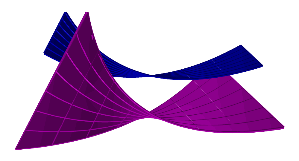
FIGURE:
A region can be extracted from a freeform surface using SREGION.
See also CREGION, TREGION, and MREGION.
SREPARAM
SurfaceType SREPARAM( SurfaceType Srf, ConstantType Direction,
NumericType MinParam, NumericType MaxParam )
or
TrimSrfType SREPARAM( TrimSrfType Srf, ConstantType Direction,
NumericType MinParam, NumericType MaxParam )
reparametrize Srf over a new domain from MinParam to MaxParam,
in the prescribed Direction. This operation does not affect the geometry
of the (trimmed) surface and only affine transforms its knot vectors. A
Bezier (trimmed) surface will automatically be promoted into a B-spline
surface by this function.
If MinParam equals MaxParam and both equates with one of the
parameterization keywords of PARAM_CENTRIP, PARAM_CENTRIP, PARAM_CHORD, or
PARAM_NIELFOL, then that parametrization is approximated for the surface, by
changing the knot sequence. Note this last operation affects the geometry
of the surface.
Example:
srf = sbspline( 2, 4,
list( list( ctlpt( E3, 0.0, 0.0, 1.0 ),
ctlpt( E2, 0.0, 1.0 ),
ctlpt( E3, 0.0, 2.0, 1.0 ) ),
list( ctlpt( E2, 1.0, 0.0 ),
ctlpt( E3, 1.0, 1.0, 2.0 ),
ctlpt( E2, 1.0, 2.0 ) ),
list( ctlpt( E3, 2.0, 0.0, 2.0 ),
ctlpt( E2, 2.0, 1.0 ),
ctlpt( E3, 2.0, 2.0, 2.0 ) ),
list( ctlpt( E2, 3.0, 0.0 ),
ctlpt( E3, 3.0, 1.0, 2.0 ),
ctlpt( E2, 3.0, 2.0 ) ),
list( ctlpt( E3, 4.0, 0.0, 1.0 ),
ctlpt( E2, 4.0, 1.0 ),
ctlpt( E3, 4.0, 2.0, 1.0 ) ) ),
list( list( KV_OPEN ),
list( KV_OPEN ) ) );
srf = sreparam( sreparam( srf, ROW, 0, 1 ), COL, 0, 1 );
ensures that the (trimmed) B-spline surface is defined over the unit size
parametric domain. See also CREPARAM, TREPARAM, and MREPARAM.
SREVERSE
SurfaceType SREVERSE( SurfaceType Srf )
or
TrimSrfType SREVERSE( TrimSrfType Srf )
reverse Srf by flipping the U and V parametric directions.
Note that the unary minus (i.e -Srf) also reverses the surface by
reversing the U parametric direction. If the surface is a trimmed surface,
the trimming curves are flipped accordingly to yield the same shape.
RevSrf = SREVERSE( Srf );
See also MREVERSE and TREVERSE.
SRF2TANS
ListType SRF2TANS( SurfaceType Srf1, SurfaceType Srf2,
NumericType SubdivTol, NumericType NumericTol )
computes the developable sheet(s) bi-tangent to given two surfaces
Srf1 and Srf2.
See MZERO for the meaning of the SubdivTol and NumerTol
tolerances.
Returns are lists, one per developable sheet, of piecewise linear
curves in E4, having two pairs of parameter values of the bi-tangent
points in the two input surfaces, in their parametric domain.
Example:
c1 = cbspline( 3,
list( ctlpt( E2, -1, -1 ),
ctlpt( E2, 1, -1 ),
ctlpt( E2, 1, 1 ),
ctlpt( E2, -1, 1 ) ),
list( kv_periodic ) );
c1 = coerce( c1, kv_open );
c2 = cbspline( 3,
list( ctlpt( E3, 0.8, -0.2, -0.3 ),
ctlpt( E3, 0.5, 0.0, -0.2 ),
ctlpt( E2, -0.45, -0.21 ),
ctlpt( E2, -0.45, 0.32 ),
ctlpt( E3, 0.5, -0.0, 0.2 ),
ctlpt( E3, 0.8, 0.28, 0.3 ) ),
list( kv_open ) );
s1 = sregion( sweepSrf( c1 * sc( 0.1 ), c2, off ), col, 0, 0.5 );
s2 = sregion( sweepSrf( c1 * sc( 0.1 ), c2, off ), col, 0.5, 1.0 );
BiTans = SRF2TANS( s1, s2, 0.1, 1e-6 );
computes the self bi-tangencies of a given bottle-like surface.
See figure for an example.
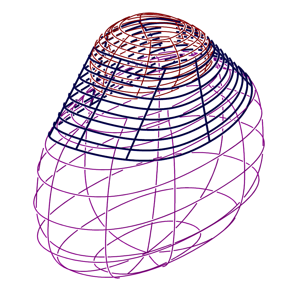
FIGURE:
Extracts self bi-tangent developable out of the given surface
using SRF2TANS.
See also SRF3TANS.
SRF3TANS
ListType SRF3TANS( ListType Srfs, NumericType Orientation,
NumericType SubdivTol, NumericType NumericTol )
computes the plane(s) tri-tangent to given three surfaces Srfs.
Srfs can be either a list of three surfaces or a list of one
surface in which self bi-tangencies are being sought.
If Orientation is 0 all tri-tangent planes are returned. Otherwise, if
Orientation equal +1 or -1, tri-tangent sheets(s)with same or different
tangency orienation are returned, respectively. See MZERO for the meaning
of the SubdivTol and NumerTol tolerances.
Returns are lists, one per developable sheet, of sample points in E6, having
three pairs of parameter values of the tri-tangent points in the three
surfaces, in their parametric domain.
Example:
c2 = cbspline( 3,
list( ctlpt( E3, 0.8, -0.2, -0.3 ),
ctlpt( E3, 0.5, 0.0, -0.2 ),
ctlpt( E2, -0.45, -0.21 ),
ctlpt( E2, -0.45, 0.32 ),
ctlpt( E3, 0.5, -0.0, 0.2 ),
ctlpt( E3, 0.8, 0.28, 0.3 ) ),
list( kv_open ) );
s1 = sFromCrvs( list( c2 * sc( 0.001 ),
c2,
c2 * tz( 1.0 ),
c2 * sc( 0.001 ) * tz( 1.0 ) ),
3, kv_open ) * sc( 0.1 );
s2 = s1 * ry( 14 ) * tx( 0.6 ) * tz( 0.02 );
s3 = s1 * rx( 12 ) * ty( 0.6 ) * tx( 0.3 ) * tz( 0.01 );
TriTans = SRF3TANS( list( s1, s2, s3 ) * sz( 1 ), 1, 0.5, -1e-6 );
Edges = nil();
for ( i = 1, 1, sizeof( TriTans ),
Pt = nth( TriTans, i ):
snoc( seval( s1, coord( Pt, 1 ), coord( Pt, 2 ) ) +
seval( s2, coord( Pt, 3 ), coord( Pt, 4 ) ), Edges ):
snoc( seval( s1, coord( Pt, 1 ), coord( Pt, 2 ) ) +
seval( s3, coord( Pt, 5 ), coord( Pt, 6 ) ), Edges ):
snoc( seval( s2, coord( Pt, 3 ), coord( Pt, 4 ) ) +
seval( s3, coord( Pt, 5 ), coord( Pt, 6 ) ), Edges ) );
computes the two outer oriented tri-tangencies to three approximate
ellipsoids. Extract and draw the two tri-tangent triangles.
See figure for an example.
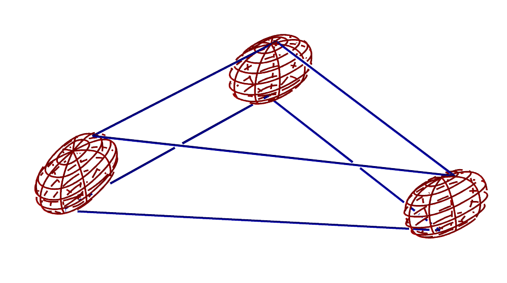
FIGURE:
Extracts tri-tangent planes out of the given three approximate
ellipsoids using SRF3TANS.
See also SRF2TANS.
SRFFFORM
ListType SRFFFORM( SurfaceType Srf, NumericType Form )
derives the four coefficients of the 1st, 2nd or 3rd surface fundamental
forms. Form can be one of 1, 2, or 3 only, designating the requested
form. Since this 2x2 matrix is symmetric, only three coefficients are
returned as a list of three scalar surfaces as (A11, A12 == A21, A22).
Example:
FFF = SRFFFORM( Srf, 1 );
SFF = SRFFFORM( Srf, 2 );
TFF = SRFFFORM( Srf, 3 );
computes the three fundamental forms of Srf.
SRFLNDST
PointType SRFLNDST( SurfaceType Srf, PointType LnPt, VectorType LnDir,
NumericType IsMinDist, NumericType SubdivTol,
NumericType NumerTol )
compute the minimal (IsMinDist TRUE) or maximal (IsMinDist FALSE)
distance betweeb surface Srf and the line defined by LnPt, a point
on the line, and LnDir, the direction of the line.
See MZERO for the meaning of the SubdivTol and NumerTol
tolerances.
Example:
Dst = SRFLNDST( Srf, LnPoint, vector( 1, 1, 1 ), TRUE, 0.1, 1e-6 );
computes the minimal distance between Srf and line LnPoint/Vector( 1, 1, 1 ).
See also SRFPTDST, CRVLNDST.
PolyType SRFKERNEL( SurfaceType Srf, NumericType Fineness,
NumericType SkipRate )
SRFKERNEL
PolyType | ListType SRFKERNEL( SurfaceType Srf | ListType SrfList,
ListType KrnlParam, NumericType Mode)
Approximates the kernel of a single surface Srf, or a list of
surfaces SrfList (only when Mode == 1). When Mode
== 0, the kernel of (a closed and continuous) surface is approximated
by deriving the parabolic points of Srf and intersecting half planes
tangent to Srf and placed at sampled set of parabolic locations.
KrnlParam is a list of control parameters and specified as
list( Fineness, SkipRate ), where Fineness governs the parabolic
curves' approximation, and SkipRate controls the sampling rate along
the parabolic curves. The function returns the list of polygons that
approximates the kernel of the surface.
When Mode == 1, the kernel of a single surface Srf, or a list
of surfaces in SrfList is computed based on derived inequality
constraints. A point P in R^3 belongs to the kernel of Srf (or
SrfList) if it satisfies the following inequalities:
> 0, for all u_i, v_i,
where S_i(u_i,v_i) is the i-th surface and N_i(u_i,v_i) is the
(inward) normal field of S_i(u_i,v_i). Starting from the bounding
box of the surface(s), this function finds the xyz sub-domains that
satisfy the above inequalities. KrnlParam is a list of control
parameters and specified as
list( SubdivTol, BoxScale, Gamma, NumTanSamples, DmnBoxOutput ),
where SubdivTol prescribes a subdivision tolerance, (non-zero)
BoxScale sets a scaling factor to size of the bounding box to compute
the kernel domains when, Gamma sets the gamma-angle for the
gamma-kernel, NumTanSamples controls the sampling rate of the tangent
planes, which are used in purging the domains during subdivision, and
DmnBoxOutput determines the form of output. The function returns a
list of kernel points if DmnBoxOutput is FALSE, and a list of the
kernel domain boxes in R3 if DmnBoxOutput is TRUE.
Example:
Krnl = SRFKERNEL( Srf, list( 0.05, 15 ), 0 );
estimates the kernel of Srf with Fineness of 0.05 and
SkipRate of 15.
Krnl = SRFKERNEL( Srf, list(0.01, 1, 0, 20, FALSE), 1 );
finds a list of points that belong to the regular kernel of Srf
by subdividing the normalized xyz domains in the bounding box of
Srf, and testing with 20 x 20 tangent planes sampled along Srf.
Krnl = SRFKERNEL( Srf, list(0.01, 1, 30, 20, FALSE), 1 );
finds a list of points that belong to the gamma-kernel of Srf
with the gamma angle of 30 degrees.
Krnl = SRFKERNEL( SrfList, list(0.01, 2.0, 0, 20, TRUE), 1 );
finds a list of kernel domains of SrfList in R3 from the
domain that has been scaled twice from the bounding box of
SrfList. 400 (20x20) tangent planes are sampled for each
surface in SrfList, to accelerate purging during subdivision.
See also CRVKERNEL.
SRFORTHONET
PointType SRFORTHONET( CurveType CrvSrc, CurveType CrvDst,
NumericType NumCrvSamples, NumericType NumLayers )
aims to approximate an orthogonal (conformal) planar (XY) mapping
bivariate surface, mapping from planar curve CrvDsrc to planar
curve SrcDst, that also must span the same domain.
Clearly, as such mapping can be quite complex, the curves better be
"well behaved" and relatively parallel to each other.
The last two parameters control the fineness of the approximation,
controlling how many samples to sample along the curves, as
NumCrvSamples, and how many layers to smaple between the curves,
as NumLayers. The more, the more accurate the result will be.
Example:
Crv1 = pcircle( vector( 0, 0, 0 ), 1 );
Crv2 = cbspline( 4,
list( ctlpt( E2, 0.7, 0.0 ),
ctlpt( E2, 0.7, 0.4 ),
ctlpt( E2, 0.1, 0.1 ),
ctlpt( E2, 0.4, 0.7 ),
ctlpt( E2, 0.0, 0.7 ) ),
list( kv_open ) );
Crv2 = crv2 +
crv2 * rz( 90 ) +
crv2 * rz( 180 ) +
crv2 * rz( 270 );
Sec = srfOrthoNet( Crv2, Crv1, 50, 50 );
creates an approximated orthogonal network, starting from crv2), toward
crv1, computing 50 layers in the approximatin and taking 50 samples along
the curves.
See also RULEDSRF.
SRFPTDST
PointType SRFPTDST( SurfaceType Srf, PointType Pt
NumericType IsMinDist, NumericType SubdivTol,
NumericType NumerTol, NumericType Cache )
compute the minimal (IsMinDist TRUE) or maximal (IsMinDist FALSE)
distance between surface Srf and point Pt.
See MZERO for the meaning of the SubdivTol and NumerTol
tolerances.
If Cache is 1, a cache of precomputed data is prepared following
by many point distance evaluations for the SAME SURFACE with Cache = 0
that take advantage of this caching, only to terminate and free the cache,
when Cache = 2.
Cache = 0 should also used when no cache is required.
Returned is the UV coordinate of the sought location on Srf.
Example:
Dst = SRFPTDST( Srf, Pt1, FALSE, 0.1, 1e-6, 0 );
computes the maximal distance between Srf and point Pt1.
See also SRFLNDST, CRVPTDST.
SRINTER
PointType SRINTER( SurfaceType Srf, PointType RayOrigin,
VectorType RayDirection, NumericType Tolerance,
NumeircType Approx )
If Approx is TRUE, computes the first intersection, if any, of the
prescribed ray originating from RayOrigin in direction RayDirection
with surface Srf.
It returns the intersection point in the parametric space of Srf with
the U and V coordinates as the X and Y coefficients of the returned value.
The intersection is computed between the ray and a polygonal approximation
of the surface Srf as set via the RESOLUTION variable.
If RayDirection is the zero vector, the closest position on Srf
to RayOrigin is returned instead.
If Approx is FALSE, the precise surface ray intersection is computed, using
an algebaric approach.
Tolerance sets the accuracy of the computation.
This function is tailored toward many invokations of ray-surface test
against the same surface. Hence, it caches local data for faster processing.
To signal the function that the processing of the current surface is
complete, use a Tolerance of zero.
Example:
RayOrigin = point( 2, 0.1, 0.3 );
RayDir = vector( -4, 0, 0 );
RayLine = coerce( RayOrigin, E3 ) + coerce( RayOrigin + RayDir, E3 );
color( RayLine, magenta );
attrib( RayLine, "dwidth", 2 );
resolution = 80;
InterPt = SRINTER( glass, RayOrigin, RayDir, 0.001 );
InterPtE3 = seval( glass, coord( InterPt, 0 ), coord( InterPt, 1 ) );
color( InterPtE3, cyan );
attrib( InterPtE3, "dwidth", 3 );
view( list( InterPtE3, RayLine, glass, axes ), 1 );
InterPt = SRINTER( glass, RayOrigin, RayDir, 0.0 );
This is a complete example of constructing a ray and intersecting it against a
surface of a glass at two different resolutions, resulting in two different
accuracies. See also RESOLUTION.
SSINTER
ListType SSINTER( SurfaceType Srf1, SurfaceType Srf2,
NumericType Euclidean, NumericType Epsilon,
NumericType Alignment )
computes the intersection curve of two surfaces, Srf1 and Srf2,
up to Epsilon accuracy. The returned data is in Euclidean space if
Euclidean is true; otherwise it is in the parametric space.
A list of two lists (for the two surfaces) of n curves each,
where n is the number of intersection curves, is returned.
If Alignment is true, the surfaces are rotated to that one bbox
of one surface whose axes are aligned, increasing the probability of detecting
disjoint cases.
Example:
s1 = sphereSrf( 0.35 ) * trans( vector( 0.0, 0.1, 0.2 ) );
s2 = coneSrf( 1, 0.5 );
Inter = nth( SSINTER( s1, s2, true, 0.1, false ), 1 );
computes the Euclidean intersection curves of a cone and a sphere,
in general positions. The Euclidean curves on the first surface are
extracted while purging the Euclidean curves on the second surface.
See also SLINTER, SCINTER, RRINTER, SSINTR2 and GGINTER.
SSINTR2
ListType SSINTR2( SurfaceType Srf1, SurfaceType Srf2,
NumericType Step, NumericType SubdivTol,
NumericType NumerTol, NumericType Euclidean,
NumericType DiscBndry )
computes the intersection curve of two surfaces, Srf1 and Srf2,
up to SubdivTol/NumerTol accuracy. The returned data is in Euclidean
space if Euclidean is true; otherwise it is in the parametric space.
Step controls the forward step size while tracing the intersection
curves.
A list of pairs of (piecewise linear) intersection curves is returned, one
for each connected component. If Euclidean is true a Euclidean curve
is also evaluated and returned.
If DiscBndry is TRUE, special case is made to properly compute
intersections along the boundary and/or along knot lines.
Example:
s1 = sphereSrf( 0.35 ) * trans( vector( 0.0, 0.1, 0.2 ) );
s2 = coneSrf( 1, 0.5 );
Inter = SSINTR2( s1, s2, 0.01, 0.01, 1e-8, false, false );
computes the intersection curves of a cone and a sphere in parameter spaces.
See also MUNIVZERO, SLINTER, SCINTER, RRINTER, SSINTER and GGINTER.
STANGENT
VectorType STANGENT( SurfaceType Srf, ConstantType Direction,
NumericType UParam, NumericType VParam,
NumericType Normalize )
or
VectorType STANGENT( TrimSrfType Srf, ConstantType Direction,
NumericType UParam, NumericType VParam,
NumericType Normalize )
compute the tangent vector to the (possibly trimmed) surface Srf at the
parameter values UParam and VParam in Direction. The
returned vector has a unit length. If Normalize TRUE, the returned
vector is normalized as well.
Example:
Tang = STANGENT( Srf, ROW, 0.5, 0.6, TRUE );
computes the unit tangent to Srf in the ROW direction at the parameter
values (0.5, 0.6).
STRIMSRF
SurfaceType STRIMSRF( TrimSrfType TSrf )
extracts the surface of a trimmed surface TSrf.
Example:
Srf = STRIMSRF( TrimSrf );
extracts the surface of TrimSrf.
See also CTRIMSRF.
STRIVAR
SurfaceType STRIVAR( TrivarType TV, ConstantType Direction,
NumericType Param ) )
extracts an iso surface from a trivariate function TV in the specified
Direction (ROW or COL or DEPTH) at the specified parameter value
Param.
Param must be contained in the parametric domain of TV in
Direction direction.
The returned surface is in the trivariate TV.
Example:
TV1 = tbezier( list( list( list( ctlpt( E3, 0.1, 0.0, 0.8 ),
ctlpt( E3, 0.2, 0.1, 2.4 ) ),
list( ctlpt( E3, 0.3, 2.2, 0.2 ),
ctlpt( E3, 0.4, 2.3, 2.0 ) ) ),
list( list( ctlpt( E3, 2.4, 0.8, 0.1 ),
ctlpt( E3, 2.2, 0.7, 2.3 ) ),
list( ctlpt( E3, 2.3, 2.6, 0.5 ),
ctlpt( E3, 2.1, 2.5, 2.7) ) ) ) );
Srf = STRIVAR( TV1, col, 0.4 );
extracts an iso surface of TV1, in the col direction at
parameter value 0.4.
See figure for an example.
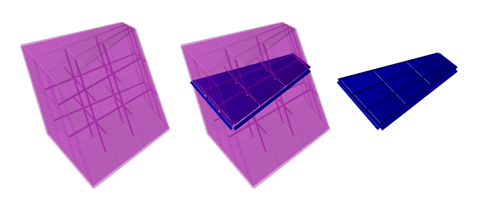
FIGURE:
Extracts an iso bilinear surface from a trilinear function,
using STRIVAR.
See also SMESH, CSURFACE, MFROMMV.
SURFPREV
SurfaceType SURFPREV( CurveType Object )
This is the same as SURFREV but approximates the surface of revolution as a
polynomial surface. The object must be a polynomial curve.
The behaviour of this function can be modified if "Rational" attribute
is provided with a non zero value to construct a precise surface of revolution
instead of a polynomial approximation.
Further if "StartAngle" and "EndAngle" are found as attributes with valid
angular prescription (in degrees), only that angular slice out of the surface
of revolution is constructed.
See also SURFREV, SURFPREV2.
SURFPREV2
SurfaceType SURFPREV2( CurveType Object,
NumericType StartAngle,
NumericType EndAngle )
This is the same as SURFPREV but also allow to specify a starting and
terminating angle.
The behaviour of this function can be modified if "Rational" attribute
is provided with a non zero value to construct a precise surface of revolution
instead of a polynomial approximation.
See also SURFREV, SURFPREV.
SURFREV
PolygonType SURFREV( PolygonType Object )
or
SurfaceType SURFREV( CurveType Object )
create a surface of revolution by rotating the first polygon/curve of the
given Object, around the Z axis. Use the linear transformation functions
to position a surface of revolution in a different orientation.
Example:
VTailAntn = SURFREV( ctlpt( E3, 0.001, 0.0, 1.0 ) +
ctlpt( E3, 0.01, 0.0, 1.0 ) +
ctlpt( E3, 0.01, 0.0, 0.8 ) +
ctlpt( E3, 0.03, 0.0, 0.7 ) +
ctlpt( E3, 0.03, 0.0, 0.3 ) +
ctlpt( E3, 0.001, 0.0, 0.0 ) );
constructs a piecewise linear B-spline curve in the XZ plane and uses it to
construct a surface of revolution by rotating it around the Z axis.
See also SURFPREV, SURFREVAXS, SURFREV2, SURFREVAX2, and TVREV.
See figure for an example.
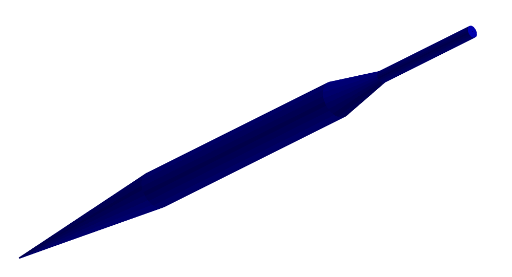
FIGURE:
A surface of revolution, VTailAntn in surfrev documentation, can be
constructed using SURFREV or SURFPREV.
SURFREVAXS
PolygonType SURFREVAXS( PolygonType Object, VectorType Axis )
or
SurfaceType SURFREVAXS( CurveType Object, VectorType Axis )
create a surface of revolution by rotating the first polygon/curve of the
given Object, around the Axis axis. Use the linear transformation
functions to position a surface of revolution in a different location.
Example:
Glass = SURFREVAXS( GCross, vector( 1, 0, 1 ) );
constructs a surface of revolution by rotating GCross around the axis of (1, 0, 1).
See also SURFPREV, SURFREV, SURFREV2, SURFREVAX2.
SURFREV2
PolygonType SURFREV2( PolygonType Object,
NumericType StartAngle,
NumericType EndAngle )
or
SurfaceType SURFREV2( CurveType Object,
NumericType StartAngle,
NumericType EndAngle )
create a surface of revolution by rotating the first polygon/curve of the
given Object, around the Z axis. The rotation does not form a complete
circle and is from the StartAngle to the EndAngle only, in degrees,
starting from the X axis toward the Y axis, in the XY plane. Use the linear
transformation functions to position a surface of revolution in a different
orientation.
Example:
Glass = SURFREV2( GCross, 45, 180 );
constructs a surface of revolution by rotating it around the Z axis from 45
to 180 degrees.
See also SURFPREV, SURFREVAXS, SURFREV, SURFREVAX2.
SURFREVAX2
PolygonType SURFREVAX2( PolygonType Object,
NumericType StartAngle,
NumericType EndAngle,
VectorType Axis )
or
SurfaceType SURFREVAX2( CurveType Object,
NumericType StartAngle,
NumericType EndAngle,
VectorType Axis )
create a surface of revolution by rotating the first polygon/curve of the
given Object, around the Axis axis. The rotation does not form
a complete circle and is from the StartAngle to the EndAngle only, in
degrees, starting from the X axis toward the Y axis, in the XY plane.
Use the linear transformation functions to position a surface of revolution
in a different location.
Example:
T4 = SURFREVAX2( PolyCross, 90, 360, vector( 1, 0, 1 ) );
constructs a polygonal surface of revolution by rotating PolygonType
PolyCross around the axis (1, 0, 1), from 45 to 180 degrees.
See also SURFPREV, SURFREVAXS, SURFREV2, SURFREV.
SVISIBLE
ListType SVISIBLE( SurfaceType Srf,
NumericType Resolution,
NumericType ConeSize )
computes a decomposition of a freeform surface Srf into regions, each
visible with a cone visibility of ConeSize degrees from one direction.
In other words, all points in one region have angular deviation of their
surface normal of less than ConeSize degrees from the set viewing
direction. Resolution controls the accuracy of the computation; the higher
this value is, more exact the result. 20 is a good starting value. Each
returned region is a trimmed surface that has a "ViewDir" attribute that
contains the viewing direction of this region.
Example:
c1 = cbezier( list( ctlpt( E3, 1.0, 0.0, 0.5 ),
ctlpt( E3, 1.1, 0.0, 0.0 ),
ctlpt( E3, 1.0, 0.0, -0.5 ) ) );
Simp = sregion( surfPRev( c1 ), col, 0.0, 1.0 ) * rz( 45 ) * rx( 90 );
Decomp = SVISIBLE( Simp, 20, 30 * pi / 180 );
SimDecomp = nil();
Mod = 5;
for ( i = 1, 1, sizeof( Decomp ),
o = nth( Decomp, i ):
v = getattr( o, "ViewDir" ):
l = ( ctlpt( E3, 0, 0, 0 ) + coerce( v, e3 ) ) * sc( 1.5 ):
j = floor( ( i - 1 ) / Mod ):
snoc( list( o, Simp, l, axes )
* view_mat * tx( ( i - 1 - j * Mod ) * 2 - 4 )
* ty( -j * 2 ),
SimDecomp ) );
view( SimDecomp, on );
decomposes a given surface Simp into regions of 30 degrees at most,
goes over the decomposed regions and orders them five in a row.
See figure for an example.
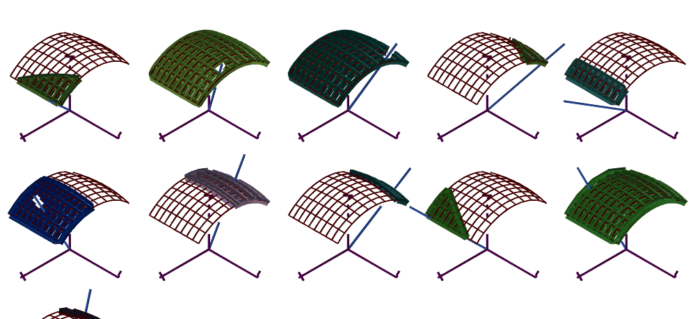
FIGURE:
A decomposition of a freeform surface into cone visible regions
of 30 degrees. The direction of visibility is also presented.
Computed using the SVISIBLE command.
SVOLUME
SurfaceType SVOLUME( SurfaceType Srf, NumericType Method, NumericType Eval )
or
NumericType SVOLUME( SurfaceType Srf, NumericType Method, NumericType Eval )
computes the integral volume surface, VSrf, of the given surface
Srf, up to a sign.
If Srf is a closed surface with domain (u0, v0) to (u1, v1), then
the difference of VSrf(u1, v1) - VSrf(u0, v0) is the requested
volume. Otherwise, the computation is for the volume occupied between the
surface Srf and the XY plane if Method equals one, and the
volume occupied between the surface Srf and the
origin if Method equals two.
If Eval is TRUE, the actual numerical value of the volume is returned.
The volume integral surface is returned if Eval is FALSE.
Example:
Spr = surfPRev( cregion( pcircle( vector( 0, 0, 0 ), 1 ), 1, 3 )
* ry( 90 ) );
SVOLUME( Spr, 1, 1 ) * 3 / 4;
SVOLUME( Spr, 2, 1 ) * 3 / 4;
are yet another two ways of approximating the value of Pi.
See also TVOLUME, SMOMENTS and CAREA.
SWEEPSRF
SurfaceType SWEEPSRF( CurveType CrossSection | ListType CrossSectionList,
CurveType Axis,
CurveType FrameCrv | VectorType FrameVec
| ConstType OFF )
constructs a generalized cylinder surface. This function sweeps a specified
cross section CrossSection along the provided Axis. If a list
of curves CrossSectionList is specified instead, the cross sections
are blended along the Axis curve so that the first/last cross section
in the list fits the first/last location on the Axis.
By default, when frame specification (third parametr) is OFF, the
orientation of the cross section is computed using the Axis curve
tangent and normal. However, unlike the Frenet frame, attempt is made to
minimize the normal change, as can happen along inflection points in the
Axis curve.
If a VectorType FrameVec is provided as a frame orientation setting,
it is used to fix the binormal direction to this value. In other words, the
orientation frame has a fixed binormal. If FrameVec has an "init"
attribute with a 1 (TRUE) value, this vector is only used as an initial
vector for the first frame, and the rest of the orientations are computed
while aiming to minimize the twist.
If a CurveType FrameCrv is specified as a frame orientation setting,
this vector field curve is evaluated at each placement of the cross section
to yield the needed binormal.
The resulting sweep is only an approximation of the real sweep. The
resulting sweep surface will not be exact, in general.
Refinement of the axis curve at the proper location, before applying
SWEEPSRF, will improve the accuracy of the output. The parametric domain
of FrameCrv does not have to match the parametric domain of Axis,
and its parametric domain is automatically made compatible by this function.
Example:
Cross = arc( vector( 0.2, 0.0, 0.0 ),
vector( 0.2, 0.2, 0.0 ),
vector( 0.0, 0.2, 0.0 ) ) +
arc( vector( 0.0, 0.4, 0.0 ),
vector( 0.1, 0.4, 0.0 ),
vector( 0.1, 0.5, 0.0 ) ) +
arc( vector( 0.8, 0.5, 0.0 ),
vector( 0.8, 0.3, 0.0 ),
vector( 1.0, 0.3, 0.0 ) ) +
arc( vector( 1.0, 0.1, 0.0 ),
vector( 0.9, 0.1, 0.0 ),
vector( 0.9, 0.0, 0.0 ) ) +
ctlpt( E2, 0.2, 0.0 );
Axis = arc( vector( -1.0, 0.0, 0.0 ),
vector( 0.0, 0.0, 0.1 ),
vector( 1.0, 0.0, 0.0 ) );
Axis = crefine( Axis, FALSE, list( 0.25, 0.5, 0.75 ) );
Srf1 = SWEEPSRF( Cross, Axis, OFF );
Srf2 = SWEEPSRF( Cross, Axis, vector( 0.0, 1.0, 1.0 ) );
Srf3 = SWEEPSRF( Cross, Axis,
cbezier( list( ctlpt( E3, 1.0, 0.0, 0.0 ),
ctlpt( E3, 0.0, 1.0, 0.0 ),
ctlpt( E3, -1.0, 0.0, 0.0 ) ) ) );
constructs a rounded rectangle cross section and sweeps it along an arc,
while orienting it several ways. The axis curve Axis is manually
refined to better approximate the requested shape.
See also SWPSCLSRF for sweep with scale.
See figure for an example.
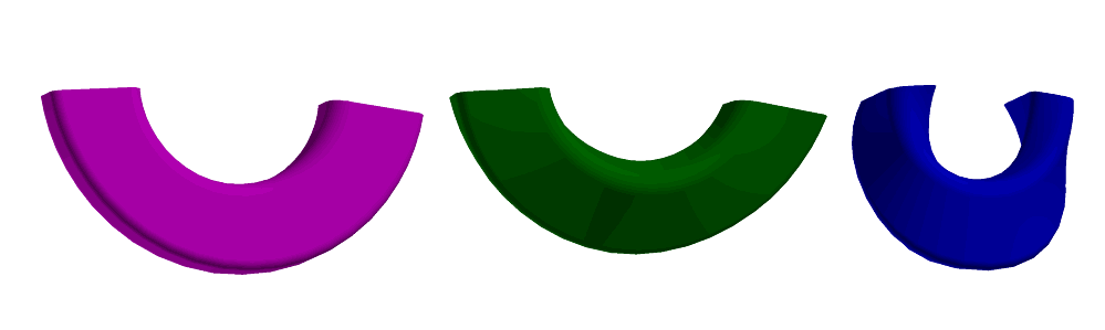
FIGURE:
Three examples of the use of SWEEPSRF (Srf1, Srf2, Srf3 from left to
right in sweepsrf documentation).
SWEEPTV
TrivarType SWEEPTV( SurfaceType CrossSection | ListType CrossSectionList,
CurveType Axis,
CurveType FrameCrv | VectorType FrameVec
| ConstType OFF )
constructs a generalized cylinder trivariate. This function sweeps a
specified cross section surface CrossSection along the provided
Axis curve.
If a list of surfaces CrossSectionList is specified instead, the
cross sections are blended along the Axis curve so that the
first/last cross section in the list fits the first/last location on the
Axis.
By default, when frame specification (third parameter) is OFF, the
orientation of the cross section is computed using the Axis curve
tangent and normal. However, unlike the Frenet frame, attempt is made to
minimize the normal change, as can happen along inflection points in the
Axis curve.
If a VectorType FrameVec is provided as a frame orientation setting,
it is used to fix the binormal direction to this value. In other words, the
orientation frame has a fixed binormal. If FrameVec has an "init"
attribute with a 1 (TRUE) value, this vector is only used as an initial
vector for the first frame, and the rest of the orientations are computed
while aiming to minimize the twist.
If a CurveType FrameCrv is specified as a frame orientation setting,
this vector field curve is evaluated at each placement of the cross section
to yield the needed binormal.
The resulting sweep is only an approximation of the real sweep. The
resulting sweep trivariate will not be exact, in general.
Refinement of the axis curve at the proper location, before applying
SWEEPTV, will improve the accuracy of the output. The parametric domains
of FrameCrv does not have to match the parametric domain of Axis,
and its parametric domain is automatically made compatible by this function.
Example:
cross = ruledSrf( 0,
arc( vector( 0.2, 0.0, 0.0 ),
vector( 0.2, 0.2, 0.0 ),
vector( 0.0, 0.2, 0.0 ) ) +
arc( vector( 0.0, 0.3, 0.0 ),
vector( 0.2, 0.3, 0.0 ),
vector( 0.2, 0.5, 0.0 ) ),
arc( vector( 0.8, 0.0, 0.0 ),
vector( 0.8, 0.2, 0.0 ),
vector( 1.0, 0.2, 0.0 ) ) +
arc( vector( 1.0, 0.3, 0.0 ),
vector( 0.8, 0.3, 0.0 ),
vector( 0.8, 0.5, 0.0 ) ) );
Axis = arc( vector( -1.0, 0.0, 0.0 ),
vector( 0.0, 0.0, 0.1 ),
vector( 1.0, 0.0, 0.0 ) );
Axis = crefine( Axis, FALSE, list( 0.25, 0.5, 0.75 ) );
TV1 = SWEEPTV( Cross, Axis, OFF );
TV2 = SWEEPTV( Cross, Axis, vector( 0.0, 1.0, 1.0 ) );
TV3 = SWEEPTV( Cross, Axis,
cbezier( list( ctlpt( E3, 1.0, 0.0, 0.0 ),
ctlpt( E3, 0.0, 1.0, 0.0 ),
ctlpt( E3, -1.0, 0.0, 0.0 ) ) ) );
constructs a rounded rectangle cross section and sweeps it along an arc,
while orienting it several ways. The axis curve Axis is manually
refined to better approximate the requested shape.
See also SWPSCLTV for sweep with scale and SWEEPSRF.
SWPSCLSRF
SurfaceType SWPSCLSRF( CurveType CrossSection | ListType CrossSectionList,
CurveType Axis, NumericType Scale | CurveType ScaleCrv,
CurveType FrameCrv | VectorType FrameVec
| ConstType OFF,
NumericType AxisRefine, NumericType C1JointType )
constructs a generalized cylinder surface. This function sweeps a specified
cross section CrossSection along the provided Axis. If a list
of curves CrossSectionList is specified instead, the cross sections
are blended along the Axis of the curve so that the first/last cross
section in the list fits the first/last location on the Axis.
The cross section may be scaled by a constant value Scale, or scaled
along the Axis parametric direction via a scaling curve ScaleCrv.
The ScaleCrv can be an E2 curve in which the X axis is ignored and the
Y axis serves to scale the cross sections along the sweep. If, however,
ScaleCrv is an E3 curve, the Y and Z coordinates of ScaleCrv
are used to scale the cross sections in X and Y, respectively. The X axis
can be used to give a visible form to ScaleCrv, to be displayed and
examined, and again, it is ignored by this function.
By default, when frame specification is OFF, the orientation
of the cross section is computed using the Axis curve tangent and
normal. However, unlike the Frenet frame, attempt is made to minimize
the normal change, as can happen along inflection points in Axis.
If a VectorType FrameVec is provided as a frame orientation setting,
it is used to fix the binormal direction to this value. In other words, the
orientation frame has a fixed binormal. If FrameVec has an "init"
attribute with a 1 (TRUE) value, this vector is only used as an initial
vector for the first frame.
If a CurveType FrameCrv is specified as a frame orientation
setting, this vector field curve is evaluated at each placement of
the cross section to yield the needed binormal.
AxisRefine an integer value to define possible refinement of the
Axis to better reflect the information in ScalingCrv and the
orientation. A value of zero will force no refinement while a value of
n > 0 will insert n times the number of control points in ScaleCrv
into Axis, better emulating the requested sweep.
If AxisRefine is negative, it is used as a positive value while a
bound on the sweep approximation error is computed and placed as "SweepError"
attribute on the result.
The resulting sweep is only an approximation of the real sweep. The
scaling and axis placement will not be exact, in general.
Manual refinement (in addition to AxisRefine) of the axis curve at
the proper location, where accuracy is important, should improve the accuracy
of the output. The parametric domains of ScaleCrv and FrameCrv do
not have to match the parametric domain of Axis, and their domains are
made compatible by this function.
If the Axis curve has C^1 discontinuities, they can be treated as
follows, depending on the value of C1JointType:
0 No treatment of C^1 discontinuities and if Axis
has a C^1 discontinuity, the function will abort.
1 Will only subdivide the Axis at all C^1 discontinuity and
compute individual sweeps for each of the continuus pieces.
2 Will attempt to round the C^1. If a polynomial sweep,
round will be approximately circular. If a rational sweep, the
round will be circular. Result will be G^1 continuous.
3 Will chamfer the corner, resulting in a C^1 discontinuous sweep.
4 Will miter the corner, resulting in a C^1 discontinuous sweep.
Example:
Cross = arc( vector( -0.11, -0.1, 0.0 ),
vector( -0.1, -0.1, 0.0 ),
vector( -0.1, -0.11, 0.0 ) ) +
arc( vector( 0.1, -0.11, 0.0 ),
vector( 0.1, -0.1, 0.0 ),
vector( 0.11, -0.1, 0.0 ) ) +
arc( vector( 0.11, 0.1, 0.0 ),
vector( 0.1, 0.1, 0.0 ),
vector( 0.1, 0.11, 0.0 ) ) +
arc( vector( -0.1, 0.11, 0.0 ),
vector( -0.1, 0.1, 0.0 ),
vector( -0.11, 0.1, 0.0 ) ) +
ctlpt( E2, -0.11, -0.1 );
scaleCrv = cbspline( 3,
list( ctlpt( E2, 0.05, 1.0 ),
ctlpt( E2, 0.1, 0.0 ),
ctlpt( E2, 0.2, 2.0 ),
ctlpt( E2, 0.3, 0.0 ),
ctlpt( E2, 0.4, 2.0 ),
ctlpt( E2, 0.5, 0.0 ),
ctlpt( E2, 0.6, 2.0 ),
ctlpt( E2, 0.7, 0.0 ),
ctlpt( E2, 0.8, 2.0 ),
ctlpt( E2, 0.85, 1.0 ) ),
list( KV_OPEN ) );
Axis = circle( vector( 0, 0, 0 ), 1 );
Frame = circle( vector( 0, 0, 0 ), 1 )
* rotx( 90 ) * trans( vector( 1.5, 0.0, 0.0 ) );
Srf1 = SWPSCLSRF( Cross, Axis, scaleCrv, off, 0, 0 );
Srf2 = SWPSCLSRF( Cross, Axis, scaleCrv, off, 2, 0 );
Srf3 = SWPSCLSRF( Cross, Axis, 1.0, Frame, 0, 0 );
constructs a rounded rectangle cross section and sweeps it along a circle,
while scaling and orienting in several ways. The axis curve Axis is
automatically refined in Srf2 to better approximate the requested
scaling.
See also SWEEPSRF for sweep with no scale.
See figure for an example.
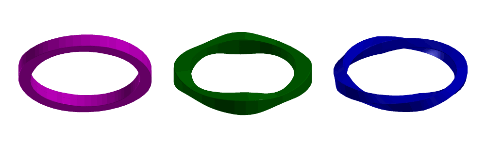
FIGURE:
Three examples of the use of SWPSCLSRF (Srf1, Srf2, Srf3 from left
to right in SWPSCLSRF documentation).
SWPSCLTV
SurfaceType SWPSCLTV( SurfaceType CrossSection | ListType CrossSectionList,
CurveType Axis, NumericType Scale | CurveType ScaleCrv,
CurveType FrameCrv | VectorType FrameVec
| ConstType OFF,
NumericType AxisRefine, NumericType C1JointType )
constructs a generalized cylinder trivariate. This function sweeps a
specified cross section CrossSection surface along the provided
Axis curve.
If a list of surfaces CrossSectionList is specified instead, the
cross sections are blended along the Axis curve so that the
first/last cross section in the list fits the first/last location on the
Axis curve.
The cross section may be scaled by a constant value Scale, or scaled
along the Axis parametric direction via a scaling curve ScaleCrv.
By default, when frame specification is OFF, the orientation
of the cross section is computed using the Axis curve tangent and
normal. However, unlike the Frenet frame, attempt is made to minimize
the normal change, as can happen along inflection points in Axis.
If a VectorType FrameVec is provided as a frame orientation setting,
it is used to fix the binormal direction to this value. In other words, the
orientation frame has a fixed binormal. If FrameVec has an "init"
attribute with a 1 (TRUE) value, this vector is only used as an initial
vector for the first frame, and the rest of the orientations are computed
while aiming to minimize the twist.
If a CurveType FrameCrv is specified as a frame orientation
setting, this vector field curve is evaluated at each placement of
the cross section to yield the needed binormal.
AxisRefine is an integer value to define possible refinement of the
Axis to better reflect the information in ScalingCrv and the
orientation frame. A value of zero will
force no refinement while a value of n > 0 will insert n times the
number of control points in ScaleCrv into Axis, better emulating
the requested sweep.
If AxisRefine is negative, it is used as a positive value while a
bound on the sweep approximation error is computed and placed as "SweepError"
attribute on the result.
The resulting sweep is only an approximation of the real sweep. The
scaling and axis placement will not be exact, in general.
Manual refinement (in addition to AxisRefine) of the axis curve at
the proper location, where accuracy is important, should improve the accuracy
of the output. The parametric domains of ScaleCrv and FrameCrv do
not have to match the parametric domain of Axis, and their domains are
made compatible by this function.
If the Axis curve has C^1 discontinuities, they can be treated as
follows, depending on the value of C1JointType:
0 No treatment of C^1 discontinuities and if Axis
has a C^1 discontinuity, the function will abort.
1 Will only subdivide the Axis at all C^1 discontinuity and
compute individual sweeps for each of the continuus pieces.
2 Will attempt to round the C^1. If a polynomial sweep,
round will be approximately circular. If a rational sweep, the
round will be circular. Result will be G^1 continuous.
3 Will chamfer the corner, resulting in a C^1 discontinuous sweep.
4 Will miter the corner, resulting in a C^1 discontinuous sweep.
Example:
cross = ruledSrf( 0,
arc( vector( 0.2, 0.0, 0.0 ),
vector( 0.2, 0.2, 0.0 ),
vector( 0.0, 0.2, 0.0 ) ) +
arc( vector( 0.0, 0.3, 0.0 ),
vector( 0.2, 0.3, 0.0 ),
vector( 0.2, 0.5, 0.0 ) ),
arc( vector( 0.8, 0.0, 0.0 ),
vector( 0.8, 0.2, 0.0 ),
vector( 1.0, 0.2, 0.0 ) ) +
arc( vector( 1.0, 0.3, 0.0 ),
vector( 0.8, 0.3, 0.0 ),
vector( 0.8, 0.5, 0.0 ) ) );
scaleCrv = cbspline( 3,
list( ctlpt( E2, 0.05, 1.0 ),
ctlpt( E2, 0.1, 0.0 ),
ctlpt( E2, 0.2, 2.0 ),
ctlpt( E2, 0.3, 0.0 ),
ctlpt( E2, 0.4, 2.0 ),
ctlpt( E2, 0.5, 0.0 ),
ctlpt( E2, 0.6, 2.0 ),
ctlpt( E2, 0.7, 0.0 ),
ctlpt( E2, 0.8, 2.0 ),
ctlpt( E2, 0.85, 1.0 ) ),
list( KV_OPEN ) );
Axis = circle( vector( 0, 0, 0 ), 1 );
Frame = circle( vector( 0, 0, 0 ), 1 )
* rotx( 90 ) * trans( vector( 1.5, 0.0, 0.0 ) );
Tv1 = SWPSCLTV( Cross, Axis, scaleCrv, off, 0, 0 );
Tv2 = SWPSCLTV( Cross, Axis, scaleCrv, off, 2, 0 );
Tv3 = SWPSCLTV( Cross, Axis, 1.0, Frame, 0, 0 );
constructs a rounded rectangle cross section and sweeps it along a circle,
while scaling and orienting in several ways. The axis curve Axis is
automatically refined in Tv2 to better approximate the requested
sweep.
See also SWEEPTV for sweep with no scale and SWPSCLSRF.
SWUNGASUM
SurfaceType SWUNGASUM( CurveType Crv1, CurveType Crv2 )
or
TrivarType SWUNGASUM( CurveType Crv, SurfaceType Srf )
Given two curves (or a curve and a surface), compute a swung surface
(trivariate) that equals:
S(r, t) = (x1(r) x2(t), x1(r) y2(t), y1(r))
or
T(u, v, w) = (Sx(v, w) Cx(u), Sx(v, w) Cy(u), Sy(v, w))
Example:
circ = circle( vector( 0.0, 0.0, 0.0 ), 1.5 ) * ry( 90 );
arc1 = arc( vector( 0.0, 1.0, 0.0 ),
vector( 0.0, 0.0, 0.0 ),
vector( 1.0, 0.0, 0.0 ) );
as1 = SWUNGASUM( circ * ry( -90 ), arc1 );
arc1 = cregion( circle( vector( 0.0, 0.0, 0.0 ), 1.5 ), 0, 2 ) * rz( 90 );
c2 = coerce( cbspline( 3,
list( ctlpt( E2, 1.0, 0.0 ),
ctlpt( E2, 0.2, 0.2 ),
ctlpt( E2, 0.0, 1.0 ),
ctlpt( E2, -0.2, 0.2 ),
ctlpt( E2, -1.0, 0.0 ),
ctlpt( E2, -0.2, -0.2 ),
ctlpt( E2, 0.0, -1.0 ),
ctlpt( E2, 0.2, -0.2 ) ),
list( KV_PERIODIC ) ),
KV_OPEN );
as2 = SWUNGASUM( arc1, c2 );
creates two algebraic sum surfaces, one in the shape of a cylinder as
a sum of a line and a circle, and one circular sweep.
See figure for an example.
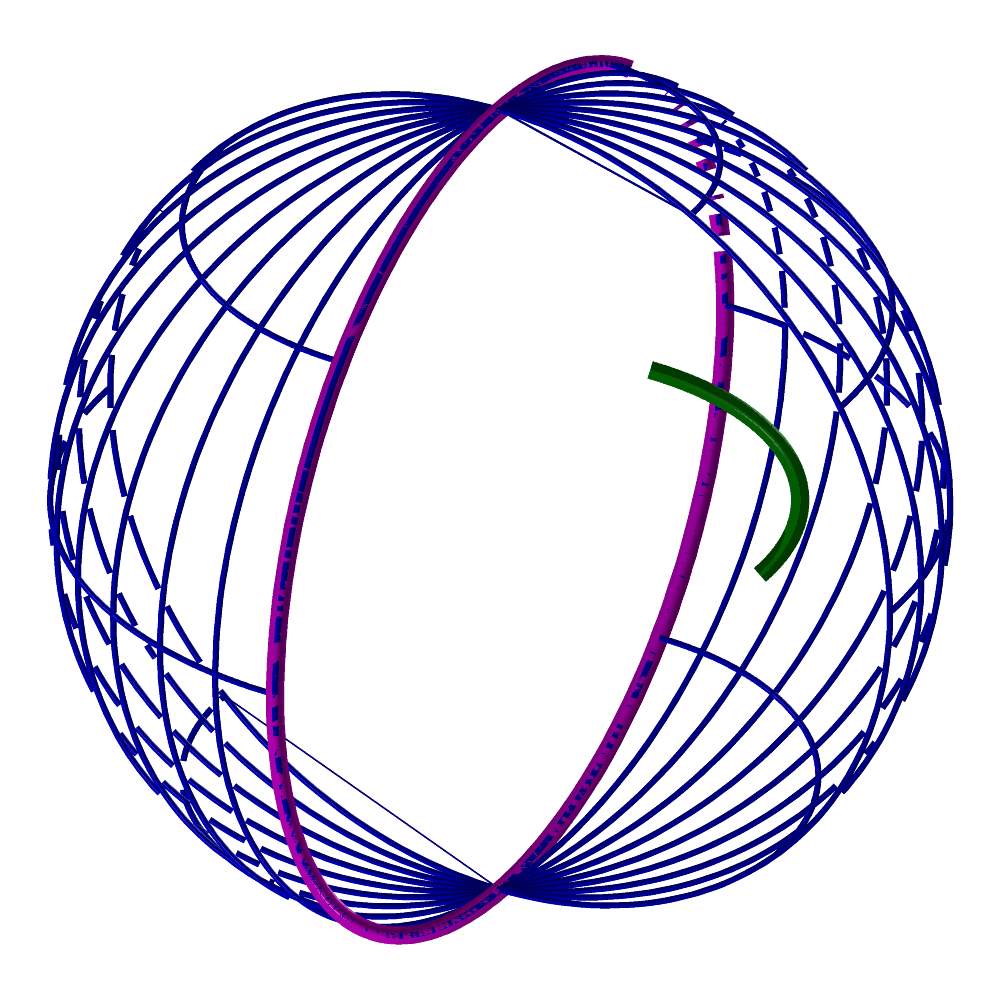
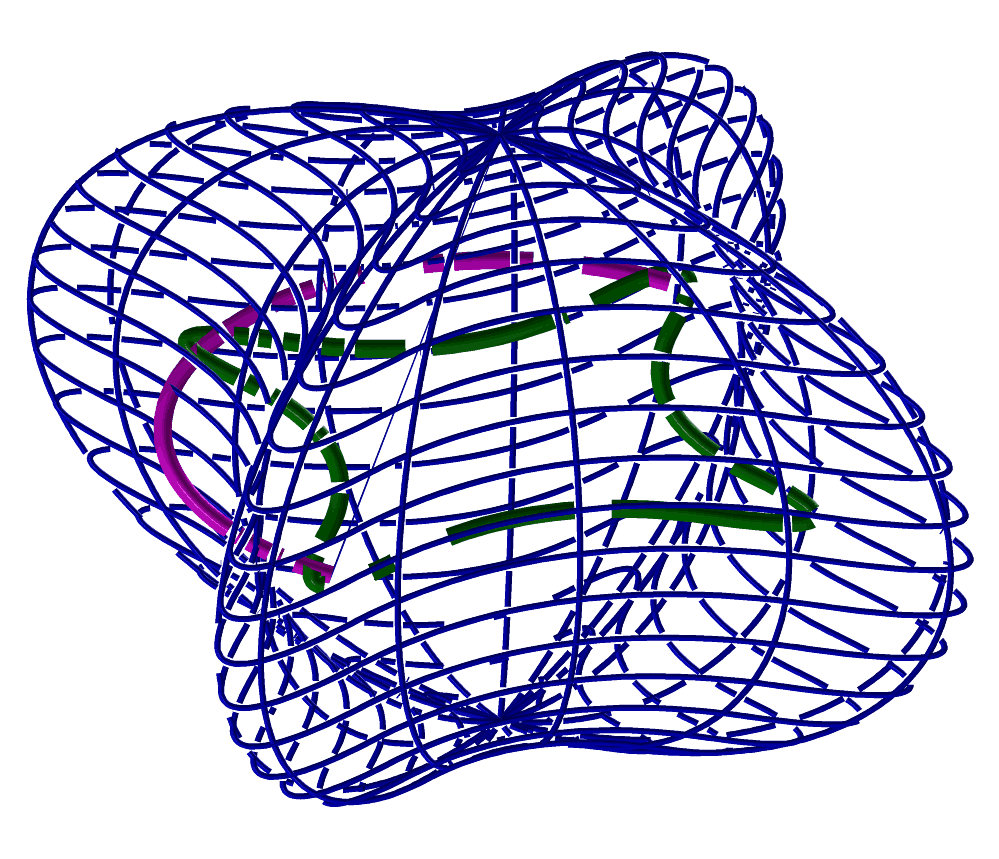
FIGURE:
An algebraic swung sum of a circle and a line creating a portion
of a sphere (left) and a general swung surface between a circle and
a periodic curve (right), both using SWUNGASUM.
SYMBCPROD
CurveType SYMBCPROD( CurveType Crv1, CurveType Crv2 )
or
SurfaceType SYMBCPROD( SurfaceType Srf1, SurfaceType Srf2 )
or
MultivarType SYMBCPROD( MultivarType MV1, MultivarType MV2 )
compute the symbolic cross product of the two given
curves/surfaces/multivariates as a curve, surface or multivariate.
Example:
NrmlSrf = SYMBCPROD( sderive( Srf, ROW ), sderive( Srf, COL ) )
computes a normal surface as the cross product of the two surface partial
derivatives (see SNRMLSRF).
See also SYMBIPROD, SYMBDPROD, SYMBPROD, SYMBSUM, SYMBDIFF.
SYMBDIFF
CurveType SYMBDIFF( CurveType Crv1, CurveType Crv2 )
or
SurfaceType SYMBDIFF( SurfaceType Srf1, SurfaceType Srf2 )
or
MultivarType SYMBDIFF( MultivarType MV1, MultivarType MV2 )
compute the symbolic difference of the two given
curves/surfaces/multivariates as a curve, surface or multivariate.
The difference is computed coordinate-wise.
Example:
DiffCrv = SYMBDIFF( Crv1, Crv2 )
DistSqrCrv = symbdprod( DiffCrv, DiffCrv )
See also SYMBCPROD, SYMBDPROD, SYMBIPROD, SYMBPROD, SYMBSUM.
SYMBDPROD
CurveType SYMBDPROD( CurveType Crv1, CurveType Crv2 )
or
CurveType SYMBDPROD( CurveType Crv1, VectorType Vec2 )
or
SurfaceType SYMBDPROD( SurfaceType Srf1, SurfaceType Srf2 )
or
SurfaceType SYMBDPROD( SurfaceType Srf1, VectorType Vec2 )
or
MultivarType SYMBDPROD( MultivarType MV1, MultivarType MV2 )
or
MultivarType SYMBDPROD( MultivarType MV1, VectorType Vec2 )
compute the symbolic dot (inner) product of the two given
curves/surfaces/multivariates as a scalar
curve/surface/multivariate. As an alternative, one parameter can
also be a regular vector.
Example:
DiffCrv = symbdiff( Crv1, Crv2 )
DistSqrCrv = SYMBDPROD( DiffCrv, DiffCrv )
computes a scalar curve that at parameter t is equal to the distance
square between Crv1 at t and Crv2.
See also SYMBCPROD, SYMBIPROD, SYMBPROD, SYMBSUM, SYMBDIFF.
SYMBIPROD
NumericType SYMBIPROD( CurveType Crv, NumericType Order1, NumericType Order2 )
or
NumericType SYMBIPROD( NumericType Dummy, NumericType Idx1, NumericType Idx2 )
compute the inner product of two B-spline basis functions. The first form
defines the function space to be the same as the function space of Crv
of order Order1 (first basis function) by Order2. The second
basis function in the inner product is defined as,
_
|
| Bi,o1(t) Bj,o2(t) dt.
|
-
The second form prescribes the indices of the two basis functions,
i and j. The first form returns zero in case of an error. The second
form returns the result of the inner product.
Example:
SYMBIPROD( Crv = pcircle( vector( 0, 0, 0 ), 1 ), 4, 4 );
for ( i = 0, 1, nth( ffmsize( Crv ), 1 ) - 1,
for ( j = 0, 1, nth( ffmsize( Crv ), 1 ) - 2,
printf( "%3.3f ", list( SYMBIPROD( 0, i, j ) ) ) ):
printf( "\n", nil() ) );
prints all possible inner products of the B-spline function space of
pcircle, of cubics vs. cubics.
See also SYMBCPROD, SYMBDPROD, SYMBPROD, SYMBSUM, SYMBDIFF.
SYMBPROD
CurveType SYMBPROD( CurveType Crv1, CurveType Crv2 )
or
SurfaceType SYMBPROD( SurfaceType Srf1, SurfaceType Srf2 )
or
MultivarType SYMBPROD( MultivarType MV1, MultivarType MV2 )
compute the symbolic product of the two given curves/surfaces/multivariates
as a curve, surface or multivariate. The product is computed coordinate-wise.
Example:
ProdSrf = SYMBPROD( Srf1, Srf2 )
See also SYMBCPROD, SYMBDPROD, SYMBIPROD, SYMBSUM, SYMBDIFF.
SYMBSUM
CurveType SYMBSUM( CurveType Crv1, CurveType Crv2 )
or
SurfaceType SYMBSUM( SurfaceType Srf1, SurfaceType Srf2 )
or
MultivarType SYMBSUM( MultivarType MV1, MultivarType MV2 )
compute the symbolic sum of the two given curves/surfaces/multivariates as
a curve, surface or multivariate. The sum is computed coordinate-wise.
Example:
SumCrv = SYMBSUM( Crv1, Crv2 )
See also SYMBCPROD, SYMBDPROD, SYMBIPROD, SYMBPROD, SYMBDIFF.
TADAPISO
CurveType TADAPISO( TrivarType TV, NumericType SrfDir, NumericType Tol,
NumericType CrvDir, NumericType CntrEps )
compute adaptive isocurves coverage for the given trivariate TV.
The coverage extracts iso-surfaces adaptively from TV in SrfDir
and then extract iso-curves adaptively from each such iso-surface in
CrvDir. If the trivariate (and hence surfaces) are trimmed,
CntrEps controls the accuracy of the trimming approximation.
SrfDir can be one of ROW, COL or DEPTH. CrvDir can be one
of COL,ROW, or 0 to return the surfaces (and no curves).
Example:
Cvr = TADAPISO( TV, col, Tol, 0, 0.01 );
to return the covering iso-surfaces of trivariate TV. See also
SADAPISO.
See figure for an example.
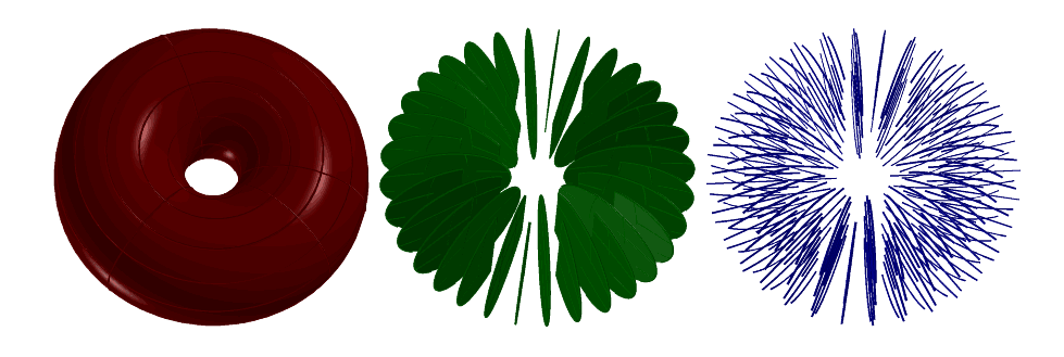
FIGURE:
Computes a coverage for a volumetric torus object by curves or
surfaces using TADAPISO.
Left shows the original volumetric model, middle shows covering by
surfaces, and right shows covering by curves.
TBEZIER
TrivarType TBEZIER( ListType CtlMesh )
creates a Bezier trivariate using the provided control mesh. CtlMesh
is a list of planes, each of which is a list of rows, each of which is a list
of control points. All control points must be of type (E1-E9, P1-P9), or
regular PointType defining the trivariate's control mesh. The surface point
type will be of a space which is the union of the spaces of all points.
Example:
TV = TBEZIER( list( list( list( ctlpt( E3, 0.1, 0.1, 0.0 ),
ctlpt( E3, 0.2, 0.5, 1.1 ),
ctlpt( E3, 0.3, 0.1, 2.2 ) ),
list( ctlpt( E3, 0.4, 1.3, 0.5 ),
ctlpt( E3, 0.5, 1.7, 1.7 ),
ctlpt( E3, 0.6, 1.3, 2.9 ) ),
list( ctlpt( E3, 0.7, 2.4, 0.5 ),
ctlpt( E3, 0.8, 2.6, 1.4 ),
ctlpt( E3, 0.9, 2.8, 2.3 ) ) ),
list( list( ctlpt( E3, 1.1, 0.1, 0.5 ),
ctlpt( E3, 1.3, 0.2, 1.7 ),
ctlpt( E3, 1.5, 0.3, 2.9 ) ),
list( ctlpt( E3, 1.7, 1.2, 0.0 ),
ctlpt( E3, 1.9, 1.4, 1.2 ),
ctlpt( E3, 1.2, 1.6, 2.4 ) ),
list( ctlpt( E3, 1.4, 2.3, 0.9 ),
ctlpt( E3, 1.6, 2.5, 1.7 ),
ctlpt( E3, 1.8, 2.7, 2.5 ) ) ) ) );
creates a trivariate Bezier which is linear in the first direction, and
quadratic in the second and third.
See figure for an example.
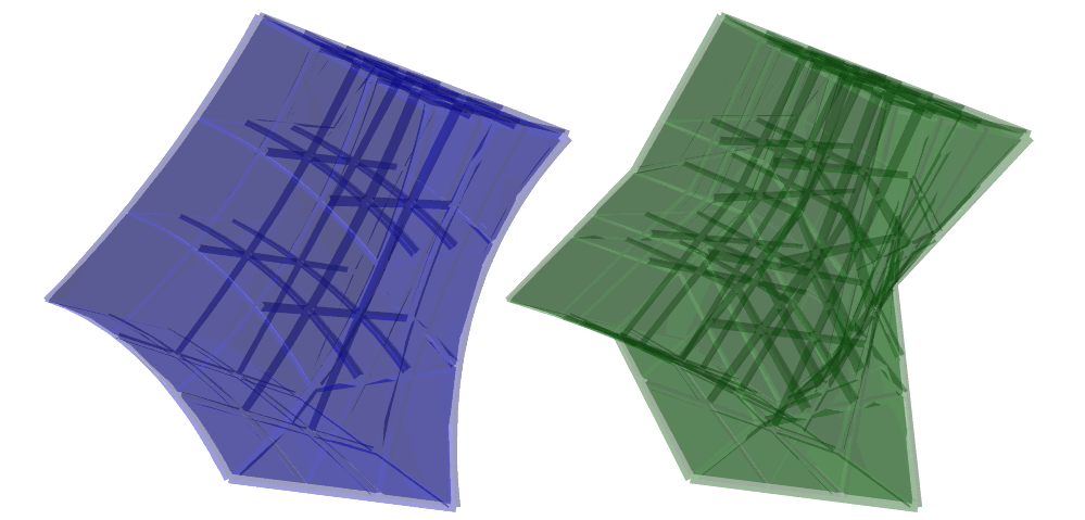
FIGURE:
A trivariate Bezier of degree 2 by 3 by 3 (left) and a trilinear
B-spline (right). Both share the same control mesh.
TBOOLONE
TrivarType TBOOLONE( SurfaceType Srf )
Given a surface closed in one direction (like a sweep of a closed curve),
the surface is subdivided into four segments in the parametric space that
are then fed into TBOOLSUM. This is useful if a volume bounded by
Srf should be "filled" abd parameterized.
Example:
Srf = TBOOLONE( CylinderSrf );
creates a cylinder volume, parameterizing the entire volume of
CylinderSrf.
See figure for an example.
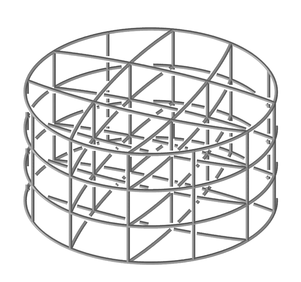
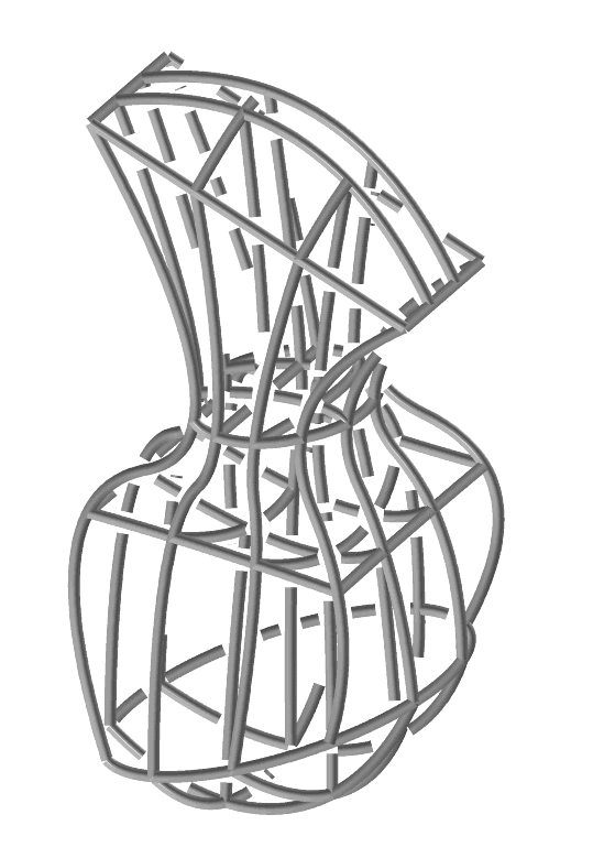
FIGURE:
A volumetric Boolean sum of a cylinder (left) using TBOOLONE
and a general volumetric Boolean sum of six surfaces (right)
using TBOOLSUM.
See also TBOOLSUM, BOOLONE.
TBOOLSUM
TrivarType TBOOLSUM( Mode,
SurfaceType Srf1, SurfaceType Srf2,
SurfaceType Srf3, SurfaceType Srf4,
SurfaceType Srf5, SurfaceType Srf6 )
The Mode parameter indicates which variant of the operator to use.
For regular Boolean sum operator, it should be 0. The regular operator
constructs a volume using the provided up to six surfaces as up to
its six boundary surfaces, forming a topology of a cube. Surfaces do
not have to have the same order or type, and will be promoted to
their least common denominator. The boundary curves of the provided
surfaces should match but the stitching will be performed
automatically so the order or orientation of all surfaces will be set
automatically to follow that of Srf1 that is not modified.
There are several options of only two input surfaces, three input
surfaces, four input surfaces or the full six surfaces, as follows:
2 srfs Constructs a trivariate TV from two input surfaces, Srf1
and Srf2 that must share a boundary C, as
TV = Srf1 + Srf2 - C;
3 srfs Constructs a trivariate TV from two input surfaces, Srf1
Srf2 and Srf3 that must share a boundaries C12, C13,
C23, as TV = Srf1 + Srf2 + Srf2 - C12 - C13 - C23 + P
where P is the common point of the three input surfaces.
4 srfs In this case full volumetric Boolean sum is computed while
Srf5 and Srf6 are derived as Boolean suum surfaces from the
boundary curves there share with the first, provided,
four surfaces.
The four surfaces must form a sleeve with two openings
for Srf5 and Srf6.
6 srfs In this case, a full volumetric Boolean sum is computed.
Surface parameters that are not provided should be specified as
non-surface parameters (i.e. 0 is this surface is not used).
For Kernel-based Boolean sum operator, which is used to construct valid
Boolean sum trivariate (i.e. with positive Jacobian throughout the domain),
theMode parameter should be a list of five numeric values:
( Op, DistRatio, Limit, SubEps, IsSingular), where
Op is either 0 or 1 for adding DOFs using degree raising or knot
insertion, respectively.
DistRatio is a number in [0, 1] to set how far to move internal
control points toward the kernel.
If 1 the points are moved to the kernel point.
Place a Limit on the number of knots to add or the maximal
degree in degree raising.
SubEps is the Subdivision epsilon. 0.01 is a reasonable start for
a unit size geometry.
IsSingular can be:
TRUE to allow singularity at the kernel point.
FALSE all the surface is regular.
Examples:
tv1 = TBOOLSUM( 0,
sregion( s, col, 0, 1 ),
sregion( s, col, 1, 2 ),
sregion( s, col, 2, 3 ),
sregion( s, col, 3, 4 ),
0, 0 );
tv2 = TBOOLSUM( 0,
sregion( s, col, 0, 1 ),
sregion( s, col, 1, 2 ),
0, 0, 0, 0 );
constructs a volume tv1 for the interior of closed surface s
(e. g. a cylinder with no caps), as will TBOOLONE when operated on
s, and constructs volume trivariate tv2 using two adjacent
faces of s. See also TBOOLONE, BOOLSUM.
TBSPLINE
TrivarType TBSPLINE( NumericType UOrder,
NumericType VOrder,
NumericType WOrder,
ListType CtlMesh,
ListType KnotVectors )
creates a B-spline trivariate with the provided UOrder, VOrder
and WOrder orders, the control mesh CtlMesh, and the three knot
vectors in KnotVectors.
CtlMesh is a list of planes, each of which is a list of rows, each
of which is a list of control points. All control points must be of point
type (E1-E9, P1-P9), or regular PointType defining the trivariate's control
mesh. Trivariate point type will be of a space which is the union of the
spaces of all points.
KnotVectors is a list of three knot vectors. Each knot vector is a
list of NumericType knots of length #CtlPtList plus the Order.
If, however, the length of the knot vector is equal to #CtlPtList +
Order + Order - 1}, the curve is assumed to be periodic.
The knot vector may also be a list of a single constant, KV_OPEN,
KV_FLOAT or KV_PERIODIC, in which a uniform knot vector with the
appropriate length and with open, floating or periodic end conditions
will be constructed automatically.
Example:
TV = TBSPLINE( 2, 2, 2,
list( list( list( ctlpt( E3, 0.1, 0.1, 0.0 ),
ctlpt( E3, 0.2, 0.5, 1.1 ),
ctlpt( E3, 0.3, 0.1, 2.2 ) ),
list( ctlpt( E3, 0.4, 1.3, 0.5 ),
ctlpt( E3, 0.5, 1.7, 1.7 ),
ctlpt( E3, 0.6, 1.3, 2.9 ) ),
list( ctlpt( E3, 0.7, 2.4, 0.5 ),
ctlpt( E3, 0.8, 2.6, 1.4 ),
ctlpt( E3, 0.9, 2.8, 2.3 ) ) ),
list( list( ctlpt( E3, 1.1, 0.1, 0.5 ),
ctlpt( E3, 1.3, 0.2, 1.7 ),
ctlpt( E3, 1.5, 0.3, 2.9 ) ),
list( ctlpt( E3, 1.7, 1.2, 0.0 ),
ctlpt( E3, 1.9, 1.4, 1.2 ),
ctlpt( E3, 1.2, 1.6, 2.4 ) ),
list( ctlpt( E3, 1.4, 2.3, 0.9 ),
ctlpt( E3, 1.6, 2.5, 1.7 ),
ctlpt( E3, 1.8, 2.7, 2.5 ) ) ) ),
list( list( KV_OPEN ),
list( KV_OPEN ),
list( KV_OPEN ) ) );
constructs a trilinear B-spline trivariate with open end conditions.
See figure for an example.
TCRVTR
TCRVTR
AnyType TCRVTR( TrivarType TV, PointType Pos, NumericType ComputeWhat )
computes differential curvature properties of an isosurface of
the given trivariate TV at the given (parameteric) location
Pos. Following the value of ComputeWhat, the result equals,
-1 Initialization (a must prelude)
0 Conclusion (a must postlude)
1 Returns a vector hold of the gradient
2 Returns a list of three vectors
equal to the Hessian of this location
3 Returns a list of two scalar values
(Principle curvatures) and two vectors
(Principal directions).
Every evaluation must start with an invocation of ComputeWhat
equal to -1 and terminate with ComputeWhat 0. In both cases, 1 is
returned in case of success.
Example:
TCRVTR( TV, point( 0, 0, 0 ), -1 ); # Prelude
Grad1 = TCRVTR( TV, point( 0, 0, 0 ), 1 );
Grad2 = TCRVTR( TV, point( 0, 0, 1 ), 1 );
Grad3 = TCRVTR( TV, point( 0, 1, 0 ), 1 );
Grad4 = TCRVTR( TV, point( 1, 0, 0 ), 1 );
TCRVTR( TV, point( 0, 0, 0 ), 0 ); #Postlude
TDEFORM
AnyType TDEFORM( GeometryType Tile, SurfaceType DeformingSrf,
NumericType UTiles, NumericType VTiles, NumericType WTiles,
NumericType FitTile, NumericType Precise,
NumericType CropBoundary )
or
AnyType TDEFORM( GeometryType Tile, TrivarType DeformingTV,
NumericType UTiles, NumericType VTiles, NumericType WTiles,
NumericType FitTile, NumericType Precise,
NumericType CropBoundary )
Tiles Tile UTiles x VTiles (x WTiles) times inside
the surface domain of DeformingSrf or the volumetric domain of
DeformingTV by compose Tile with DeformingSrf or
DeformingTV.
Result is precisely deformed, using composition, if Precise,
where the Tile can be almost any geometric type (a curve, a (trimmed)
surface, etc.).
If Tile is a surface, DeformingSrf must be a Bezier surface.
Result is approximated if DeformingTV and Precise is 0, by
mapping only (control) points through the trivariate. If Precise is
POSITIVE and Tile is either a curve or a (trimmed) surface, the
computation will indeed be precise using composition. If Precise is
1, the precise computation will generate as compact as possible representation
for the result while if >1, the precise result will be computed faster but not
as compact.
The Tile is supposed to span [0, 1]^2 or [0, 1]^3. If
FitTile is 2, the Tile is first fitted into the DeformingSrf/TV
domain. If FitTile is 1, the Tile is first scaled to fit as many
times as needed in the [0, 1]^3 domain and if FitTile is 0, no
Tile fitting/scaling is conducted.
If CropBoundary positive, the tiles near the boundary are cropped
that amount, assuming tile spans [0, 1]^3.
Example:
Geom = TDEFORM( Tubes, TV, 2, 2, 4, FALSE, FALSE, 0.0 );
See figure for an example.
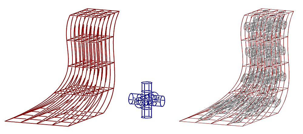
FIGURE:
Geometry can be composed into trivariate volumetric splines using
the TDEFORM command. Here, three orthogonal tubes (middle) are
composed into a trivariate (left) 2x2x4 times, yeilding the approximated
result on the right.
See also SDDMMAP, TEXTWARP, MICROSTRCT, MICROTILE,
TDERIVE
TrivarType TDERIVE( TrivarType TV, NumericType Dir )
Returns a vector field trivariate representing the differentiated
trivariate in the given direction (ROW, COL, or DEPTH). Evaluation of the
returned trivariate at a given parameter value will return a vector
representing the partial derivative of TV in Dir at that
parameter value.
TV = tbezier( list( list( list( ctlpt( E1, 0.1 ),
ctlpt( E1, 0.2 ) ),
list( ctlpt( E1, 0.3 ),
ctlpt( E1, 0.4 ) ) ),
list( list( ctlpt( E1, 2.4 ),
ctlpt( E1, 2.2 ) ),
list( ctlpt( E1, 2.3 ),
ctlpt( E1, 2.1 ) ) ) ) );
DuTV = TDERIVE( TV, ROW );
DvTV = TDERIVE( TV, COL );
DwTV = TDERIVE( TV, DEPTH );
computes the gradiate of a scalar trivariate field, by computing its
partials with respect to u, v, and w.
See also CDERIVE, SDERIVE, and MDERIVE.
TDIVIDE
TrivarType TDIVIDE( TrivarType TV, ConstantType Direction,
NumericType Param )
or
VModelType TDIVIDE( VModelType VMdl, ConstantType Direction,
NumericType Param )
Subdivides a (trimmed in case of VModelType) trivariate into two at the
specified parameter value Param in the specified Direction
(ROW, COL, or DEPTH). TV can be either a B-spline trivariate in which
Param must be contained in the parametric domain of the trivariate,
or a Bezier trivariate in which Param must be in the range of zero to
one.
If input is a VModel, it must be a VModel of a single VElement or a single
trimmed trivariates.
It returns a list of the two sub-(trimmed-)trivariates. The individual
(trimmed) trivariates may be extracted from the list using the NTH
command.
Example:
TvDiv = TDIVIDE( Tv2, depth, 0.3 );
Tv2a = nth( TvDiv, 1 ) * tx( -2.2 );
Tv2b = nth( TvDiv, 2 ) * tx( 2.0 );
subdivides Tv2 at the parameter value of 0.3 in the DEPTH direction,
See figure for an example.
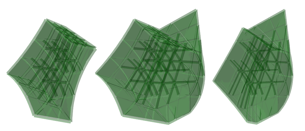
FIGURE:
A trivariate can be subdivided into two distinct regions using
TDIVIDE.
See also CDIVIDE, SDIVIDE, and MDIVIDE
TEDITPT
TrivarType TEDITPT( TrivarType TV, CtlPtType CPt, NumericType UIndex,
NumericType VIndex )
NumericType WIndex )
Provides a simple mechanism to manually modify a single control point number
UIndex, VIndex and WIndex (base count is 0) in the control mesh
of Srf by substituting CtlPt instead. CtlPt must have the same
point type as the control points of Srf. Original surface Srf is
not modified.
Example:
CPt = ctlpt( E3, 1, 2, 3 );
NewTV = TEDITPT( TV, CPt, 0, 0, 0 );
constructs a NewTV with the first control point of TV being
CPt.
TEVAL
CtlPtType TEVAL( TrivarType TV,
NumericType UParam,
NumericType VParam,
NumericType WParam )
Evaluates the provided Trivariate TV at the given UParam,
VParam and WParam values. UParam, VParam,
WParam must be contained in the surface parametric domain if TV
is a B-spline trivariate, or between zero and one if TV is a Bezier
trivariate. The returned control point has the same type as the control
points of TV.
Example:
CPt = TEVAL( TV1, 0.25, 0.22, 0.7 );
evaluates TV at the parameter values of (0.25, 0.22, 0.7).
See also CEVAL, SEVAL, MEVAL.
TEXT2GEOM
CurveType TEXT2GEOM( StringType Text, StringType Font,
NumericType FontStyle, NumericType SpaceWidth,
NumericType EdgeType3D, ListType Setup3D,
NumericType Tolerance, NumericType OutputType )
Synthesizes geometry that represents Text in one long line.
The font that is used to synthesized the text is an outline font Font,
whereas under windows Font simple lists the font name (i.e.
"Times New Roman") and under other system Font specifies the
full path of an outline ttf font file.
FontStyle selects regular font if 0, italics if 1, bold if 2,
and italic bold if 3. Might be ignored if specific font does not support
the specific style.
SpaceWidth controls the space between different characters.
EdgeType3D sets for 3D text syntehsis, the edge style than can be one
of regular if 1, chamfered if 2 or rounded if 3. Ignored for 2D text.
If 3D text generated is chamfered, Setup3D sets a 2D vector that
controls the chamfering offset amount. If swept tubes, the first parameter
of Setup3D sets the tubes radius.
If solid text is to be generated, Tolerance controls the accuracy
of the polygonal approximations.
OutputType selects the type of output geometry to create: 0 for
Bezier curves, 1 for B-spline curves, 2 for 2D solid text, 3 for 2D solid
text with outline B-spline curves, 4 for solid 3D polygonal text, 5 for
2D trimmed surfaces text, 6 for 3D trimmed surfaces text, and 7 for swept
tubes through the curves.
Example:
Text = TEXT2GEOM( "This is a test example of some 3D text",
"Times New Roman",
0, 0, 2, list( 0.01, 0.1 ), 0.001, 1 );
See figure for an example.

FIGURE:
Outline fonts can be used to synthesize text geometry, using the TEXT2GEOM
command.
See also TEXTLAYSHP, TEXTGEOM, and TEXTWARP.
TEXTLAYSHP
CurveType TEXTLAYSHP( StringType Text, StringType Font,
NumericType FontStyle, NumericType Size,
NumericType Space, NumericType Tolerance
NumericType EdgeType3D, NumericType Setup3D,
NumericType AlignmentType, NumericType OutputType,
PolyType BoundingRegion )
or
CurveType TEXTLAYSHP( StringType Text, StringType Font,
NumericType FontStyle, NumericType Size,
VectorType Space, NumericType Tolerance
NumericType EdgeType3D, NumericType Setup3D,
NumericType AlignmentType, NumericType OutputType,
CurveType BoundingRegion )
Synthesizes geometry that represents Text inside BoundingRegion.
The font that is used to synthesized the text is an outline font Font,
whereas under windows Font simple lists the font name (i.e.
"Times New Roman") and under other system Font specifies the
full path of an outline ttf font file.
FontStyle selects regular font if 0, italics if 1, bold if 2,
and italic bold if 3. Might be ignored if specific font does not support
the specific style.
Size simply scales the text.
Space is a vector of size three: (WordWidth, SpaceWidth, LineHeight),
controling the space between different words, characters, and lines,
respectively.
If solid text is to be generated, Tolerance controls the accuracy
of the polygonal approximations.
EdgeType3D sets for 3D text syntehsis, the edge style than can be one
of regular if 1, chamfered if 2 or rounded if 3. Ignored for 2D text.
If 3D text generated is chamfered, Setup3D sets a 2D vector that
controls the chamfering offset amount. If swept tubes, the first parameter
of Setup3D sets the tubes radius.
AlignmentType selects the type of text alignments: 0 for left, 1 for
center, 2 for right, and 3 for wide (full width) alignments.
OutputType selects the type of output geometry to create: 0 for
Bezier curves, 1 for B-spline curves, 2 for 2D solid text, 3 for 2D solid
text with outline B-spline curves, 4 for solid 3D polygonal text, 5 for
2D trimmed surfaces text, 6 for 3D trimmed surfaces text, and 7 for swept
tubes through the curves.
Example:
Heart = cbspline( 4,
list( ctlpt( E2, 0, 0.6 ),
ctlpt( E2, 0.2, 1 ),
ctlpt( E2, 1, 1 ),
ctlpt( E1, 1.2 ),
ctlpt( E2, 0.8, -0.6 ),
ctlpt( E2, 0, -1 ),
ctlpt( E2, 0, -1 ),
ctlpt( E2, -0.8, -0.6 ),
ctlpt( E1, -1.2 ),
ctlpt( E2, -1, 1 ),
ctlpt( E2, -0.2, 1 ),
ctlpt( E2, 0, 0.6 ) ),
list( kv_open ) ) * sc( 10 );
Str = "This is a test example of some 3D text. ";
text = TextLayShp( Str + Str + Str + Str + Str + Str + Str + Str,
"Courier New",
2, 0.67, list( 35, 10, 34 ), 0.001, 0,
list( 0.01, 0.5 ), 3, 1, Heart );
See figure for an example.
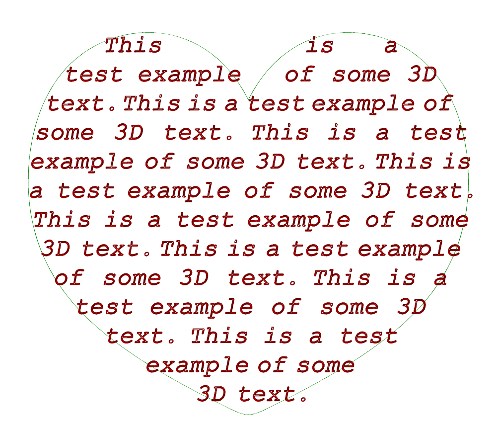
FIGURE:
Outline fonts can be used to synthesize text geometry and confine it
to arbitrary 2D shaped boundary, using the TEXTLAYSHP
command.
See also TEXT2GEOM, TEXTGEOM, and TEXTWARP.
TEXTGEOM
AnyType TEXTGEOM( StringType Str, VectorType Spacing, NumericType Scaling )
Creates a displayable geometry that represents the text in Str, with
Spacing space between individual characters. Each character is scaled
by Scaling where scaling of one generates a close to unit size
character.
Example:
a = TEXTGEOM("Text", vector( 0.12, 0, 0 ), 0.1 );
b = TEXTGEOM("IRIT", vector( 0, -0.12, 0 ), 0.1 );
Creates a horizontal Text and a vertical top to bottom IRIT,
both as geometrical objects. See TEXTWARP, TEXTLAYSHP, TEXT2GEOM and
IRITSTATE's "LoadFont" state variable.
TEXTWARP
AnyType TEXTWARP( Surface Srf, StringType Text, NumericType HSpace,
NumericType VBase, NumericType VTop, NumericType Ligature )
Warps the given text, Text, using surface Srf as warping
function with HSpace setting the horizontal spacing between
characters, VBase and VTop controls the vertical spacing
of the characters in Srf, and Ligature, if not zero, sets
the amount to contract the distance between two adjacent characters.

FIGURE:
Font and text warping using the TEXTWARP function.
Example:
c = cbezier( list( ctlpt( e2, -1.5, -0.5 ),
ctlpt( e2, -2, 0 ),
ctlpt( e2, -1, 1 ),
ctlpt( e2, 0, -2 ),
ctlpt( e2, 1, 0 ) ) );
s = sreparam( ruledSrf( 0, c, offset( c, -0.4, 0.02, off ) ), col, 0, 6 );
Txt = TEXTWARP( s, "Text Warping Toolkit", 0.08, 0.25, 0.75, 0 );
See also TEXTGEOM, TEXTLAYSHP, TEXT2GEOM and IRITSTATE's
"LoadFont" state variable.
TFROMSRFS
TrivarType TFROMSRFS( ListType SrfList, NumericType OtherOrder,
NumericType OtherEndCond )
or
TrivarType TFROMSRFS( ListType SrfList, NumericType OtherOrder,
ListType OtherKnotVector )
Constructs a trivariate by substituting the surfaces in SrfList as
planes in a control mesh of a trivariate. Surfaces in SrfList are
made compatible by promoting Bezier surfaces to B-splines if necessary,
and raising degree and refining as required before substituting the
control meshes of the surfaces as planes in the mesh of the trivariate.
The other, third, direction order is controlled by OtherOrder and
OtherEndCond. OtherOrder cannot be larger than the number of
surfaces, and OtherEndCond prescribes the desired end conditions as
one of KV_OPEN, KV_FLOAT or KV_PERIODIC, or an
explicitly prescribed knot vector OtherKnotVector.
The trivariate interpolates the first and last surfaces only.
Example:
s1 = sbezier( list( list( ctlpt( E3, -0.5, -0.5, 0 ),
ctlpt( E3, -0.5, 0.5, 0 ) ),
list( ctlpt( E3, 0.5, -0.5, 0 ),
ctlpt( E3, 0.5, 0.5, 0 ) ) ) ) * sc( 0.3 );
Srfs = list( s1 * sc( 2.0 ),
s1 * sx( 1.4 ) * ry( 45 ) * tz( 1.0 ),
s1 * ry( 90 ) * trans( vector( 1.0, 0.0, 1.1 ) ),
s1 * sx( 1.4 ) * ry( 135 ) * trans( vector( 2.0, 0.0, 1.0 ) ),
s1 * sc( 2.0 ) * ry( 180 ) * trans( vector( 2.0, 0.0, 0.0 ) ) );
color( Srfs, red );
ts = TFROMSRFS( Srfs, 3, kv_open );
color( ts, green );
view( list( Srfs, ts ), on );
Constructs a trivariate from five planar surfaces and displays both the
trivariate and the five planar surfaces, in different colors.
See figure for an example.
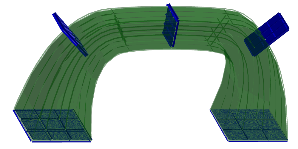
FIGURE:
A trivariate (thin lines) is constructed via five planar surfaces
(thick lines) using the TFROMSRFS constructor...
See also EXTRUDE, RULEDTV, SFROMCRVS, TINTPSRFS.
TILEPACK
TrivarType TILEPACK( AnyType Tile, ListType StepsMin, ListType StepsMax,
VectorType DomainMin, VectorType DomainMax,
NumericType IncludePartial, MergeNeighbors )
computes a tiling of some planar XY domain by periodic Tile.
Tile must hold "veci" attributes, i = 1,2, to set the
duplication directions and amounts. Default, if no "veci"
attributes, is X and Y. StepsMin and StepsMax are
explicit setting of the number of time to tile (duplicate tiles)
along "veci", backward and forward. StepsMin and StepsMax
are optional and can be nil() in which case tiling is performed until
the domain set by DomainMin and DomainMax is filled.
IncludePartial controls how to treat tiles that cross
and intersect with the boundary of the domain: 0 to exclude such tiles,
1 to include intersecting tiles, 2 to include all placements of the tile
regardless of boundaries, 3 to include all created tiles (ignores domain
clipping, and 4 to include all boundary intersecting tiles that their
centroids are inside the domain (useful when creating periodic tilings).
If MergeNeighbors is TRUE, mark the neighbors tiles with the
same ID and same RGB Attribute. Relevant only for rectangular tiles.
At least two steps in Y are needed to merge neighboring tile parts.
Example:
attrib( Tile, "vec1", vector( 0.15, 0, 0 ) ):
attrib( Tile, "vec2", vector( 0.03, 0.15, 0 ) ):
Pck1 = Tilepack( Tile, nil(), nil(),
vector( -1, -1, 0 ), vector( 1, 1, 0 ), 0, 0 ):
tiles domain [-1, 1]^2 using Tile with tiling that is not with
orthogonal directions.
See figure for an example.
FIGURE:
Tiling a 2D domain with arbitrary tile shapes can be achieved via
the TILEPACK constructor.
TINTERP
TrivarType TINTERP( TrivarType TV,
NumericType ULength, NumericType VLength, NumericType WLength,
NumericType UOrder, NumericType VOrder, NumericType WOrder );
or
TrivarType TINTERP( ListType PtList,
NumericType ULength, NumericType VLength, NumericType WLength,
NumericType UOrder, NumericType VOrder, NumericType WOrder );
Given a trivariate data structure or a list of points in R3, the above
computes a fitted trivariate in the prescribed function space (i.e.
U/V/WLength and U/V/WOrder) that interpolates/least squares approximates the
given trivariate, TV, at the node parameter values.
PtList is a list of points in Rn, n > 3. The first three coordinates
of each points in PtList prescribes the (u, v, w) parametric value and
the rest, the interpolation values. To construct a mapping from R3 to R3,
the points of PtList should be in R6. To construct a scalar trivariate
function, R4 points are expected. The (u, v, w) points are assumed to be
containted in a unit curve paramteric space - zero to one in all three
dimensions.
If U/V/WOrder are zero and the first parameter is a trivariate, the
respective order is taken for TV.
If U/V/WLength are zero and the first parameter is a trivariate, the
respective length is taken for TV.
Example:
tv = tbspline( 3, 3, 2,
list( list( list( ctlpt( E3, 0.1, 0.1, 0.0 ),
ctlpt( E3, 0.2, 0.5, 1.1 ),
ctlpt( E3, 0.3, 0.1, 2.2 ) ),
list( ctlpt( E3, 0.4, 1.3, 0.5 ),
ctlpt( E3, 0.5, 1.7, 1.7 ),
ctlpt( E3, 0.6, 1.3, 2.9 ) ),
list( ctlpt( E3, 0.7, 2.4, 0.5 ),
ctlpt( E3, 0.8, 2.6, 1.4 ),
ctlpt( E3, 0.9, 2.8, 2.3 ) ) ),
list( list( ctlpt( E3, 1.1, 0.1, 0.5 ),
ctlpt( E3, 1.3, 0.2, 1.7 ),
ctlpt( E3, 1.5, 0.3, 2.9 ) ),
list( ctlpt( E3, 1.7, 1.2, 0.0 ),
ctlpt( E3, 1.9, 1.4, 1.2 ),
ctlpt( E3, 1.2, 1.6, 2.4 ) ),
list( ctlpt( E3, 1.4, 2.3, 0.9 ),
ctlpt( E3, 1.6, 2.5, 1.7 ),
ctlpt( E3, 1.8, 2.7, 2.5 ) ) ),
list( list( ctlpt( E3, 2.8, 0.1, 0.4 ),
ctlpt( E3, 2.6, 0.7, 1.3 ),
ctlpt( E3, 2.4, 0.2, 2.2 ) ),
list( ctlpt( E3, 2.2, 1.1, 0.4 ),
ctlpt( E3, 2.9, 1.2, 1.5 ),
ctlpt( E3, 2.7, 1.3, 2.6 ) ),
list( ctlpt( E3, 2.5, 2.9, 0.7 ),
ctlpt( E3, 2.3, 2.8, 1.7 ),
ctlpt( E3, 2.1, 2.7, 2.7 ) ) ) ),
list( list( KV_OPEN ),
list( KV_OPEN ),
list( KV_OPEN ) ) );
tvi = TINTERP( tv, 0, 0, 0, 0, 0, 0 );
creates a quadratic by quaratic by linear trivariate tvi that
interpolates the control points of tv at the node parameter values.
TINTPSRFS
TrivarType TINTPSRFS( ListType SrfList, NumericType OtherOrder,
NumericType OtherEndCond, NumericType OtherParam )
constructs a trivariate by interpolating the surfaces in SrfList.
The other, third, direction order is controlled by OtherOrder and
OtherEndCond. OtherOrder cannot be larger than the number of
surfaces, and OtherEndCond prescribes the desired end conditions as
one of KV_OPEN, KV_FLOAT or KV_PERIODIC. Finally,
OtherParams affects the third direction's parameterization and can
be one of PARAM_CENTRIP, PARAM_CENTRIP, PARAM_CHORD, or
PARAM_NIELFOL.
Example:
s1 = sbezier( list( list( ctlpt( E3, -0.5, -0.5, 0 ),
ctlpt( E3, -0.5, 0.5, 0 ) ),
list( ctlpt( E3, 0.5, -0.5, 0 ),
ctlpt( E3, 0.5, 0.5, 0 ) ) ) ) * sc( 0.3 );
Srfs = list( s1 * sc( 2.0 ),
s1 * sx( 1.4 ) * ry( 45 ) * tz( 1.0 ),
s1 * ry( 90 ) * trans( vector( 1.0, 0.0, 1.1 ) ),
s1 * sx( 1.4 ) * ry( 135 ) * trans( vector( 2.0, 0.0, 1.0 ) ),
s1 * sc( 2.0 ) * ry( 180 ) * trans( vector( 2.0, 0.0, 0.0 ) ) );
color( Srfs, red );
ts = TINTPSRFS( Srfs, 3, kv_open, param_uniform );
color( ts, green );
view( list( Srfs, ts ), on );
Interpolates a trivariate thtough five planar surfaces and displays both
the trivariate and the five planar surfaces, in different colors.
See also EXTRUDE, RULEDTV, SFROMCRVS, TFROMSRFS.
TMORPH
TrivarType TMORPH( TrivarType TV1, TrivarType TV2, NumericType Blend )
creates a new trivariate which is a convex blend of the two given
trivariates. The two given trivariates must be compatible (see FFCOMPAT)
before this blend is invoked. This isv ery useful if a sequence that "morphs"
one trivariate to another is to be created and in combination with MRCHCUBE.
Example:
Size = 0.05;
for ( i = 0, step, 1.0,
Tv = TMORPH( Tv1, Tv2, i ):
view( mrchcube( list( Tv, 1, off ),
point( Size, Size, Size ), 1, IsoVal ), on ) );
creates a sequence of 1/step trivariates, morphed from Tv1 to Tv2
and displays an extracted iso surface at level IsoVal.
See also MRCHCUBE, PMORPH, CMORPH and SMORPH.
TNSCRCR
ListType TNSCRCR( PointType Cntr1, NumericType Rad1,
PointType Cntr2, NumericType Rad2, NumericType OuterTans )
computes the two outer, if OuterTans TRUE, or the two inner
if OuterTans FALSE, bi-tangents between the prescribed two circles.
Note the bi-tangents might no exist of one circle is containt in the other.
Example:
T1 = TnsCrCr( point( -2, 0.3, 0 ), 0.7, point( 1, 0, 0 ), 1, 0 );
T2 = TnsCrCr( point( -2, 0.3, 0 ), 0.7, point( 1, 0, 0 ), 1, 1 );
See also CRC2CRVTAN, CRV2TANS, CRVC1RND, SKEL2DINT.
TOFFSET
ListType TOFFSET( CurveType Crv, CurveType OffCrv, ListType Params )
or
ListType TOFFSET( SurfaceType Srf, SurfaceType OffSrf, ListType Params )
Trims local and global self intersections in curve OffCrv (surface
OffSrf) that is an offset approximation to curve Crv (surface
Srf) with parameters Params as follows:
For curves, Params contains the 4 paramers (Method, SubdivTol, TrimAmount,
NumerTol) stating with the Method of trimming which can be 1 of distance map
trmming or 2 for self intersection via uv-elimination. 2nd paramter is the
tolerance of the subdivision search, 3rd is the trimming amount which should
be a tad below the offset distance and the last parameter is a numerical
tolerance to improve trimmed locations.
For surfaces Params hold 6 parameters (TrimAmount, Validate,
Euclidean, SubdivTol, NumerTol, NumerImprove). The TrimAmount is
again a tad below the offset distance, Validate is a boolean to
activate the filering of self intersecting regions, Euclidean sets
the output form to be in Euclidean or parametric space and SubdivTol
and NumerTol are used by the multivariate solver. Finally, NumerImprove
TRUE if a final numerical improvement step is to be apllied to the result
for a better quality result.
Example:
c0 = cbspline( 3,
list( ctlpt( E2, -1, 3 ),
ctlpt( E2, -0.3, 0 ),
ctlpt( E2, 0.3, 0 ),
ctlpt( E2, 1, 3 ) ),
list( kv_open ) );
for ( i = -5, 1, 5,
if ( i != 0,
ofst = 0.15 * i:
co = offset( c0, ofst, 0.0001, off ):
none = TOFFSET( c0, co, list( 1, 0.01, abs( ofst * 0.999 ), 1e-6 ) ):
color( none, i + 6 ):
viewobj( none ) ) );
approximates several offset curves at offset amounts of 0.15 * i to
curve c0 and trim the self intersections detected in them.
See figure for an example.
FIGURE:
Properly trimmed offsets could be created using the TOFFSET function.
See also OFFSET, COFFSET, AOFFSET, LOFFSET, and MOFFSET.
PolyType TOOLSWEP( CurveType ToolProfile,
PointType ToolOrigin,
StringType MotionData,
NumericType DexelGridType,
PointType GridOrigin,
PointType GridEnd,
NumericType NumDexel0,
NumericType NumDexel1,
SurfaceType StockSurface,
NumericType RectStockTopLevel,
NumericType RectStockBotLevel,
StringType OutputSavePath )
or
PolyType TOOLSWEP( CurveType ToolProfile,
PointType ToolOrigin,
ListType MotionData,
NumericType DexelGridType,
PointType GridOrigin,
PointType GridEnd,
NumericType NumDexel0,
NumericType NumDexel1,
SurfaceType StockSurface,
NumericType RectStockTopLevel,
NumericType RectStockBtmLevel,
StringType OutputSavePath )
Performs multi-axis CNC machining simulation by computing the swept
volume of the given tool along the given path and subtracting the
same from the stock. The axis-symmetric tool is specified by ToolProfile} which is assumed to be a curve in XZ plane. The origin
of the tool is given by ToolOrigin. The motion is specified by
a sequence of positions and orientations of the tool which are
interpolated using SLERP. The motion may be speficied in a text file
MotionData with each line containing a space-separated
six-tuple specifying position and orientation of the tool, or a list
of list of six-tuples. The stock is represented using a
dexel-grid. The parameter DexelGridType may take values 0, 1 or
2 to imply dexels along the X, Y or Z axis. The origin and the end of
the grid are given by GridOrigin and GridEnd
respectively. The number of dexels in the two directions are given by
NumDexel0 and NumDexel1. The dexel grid representation of
the stock may be computed either from StockSurface which is a
closed surface, or from RectStockTopLevel and RectStockBtmLevel} which specify the top and the bottom levels of a
rectangular stock. The intermediate output may be saved at OutputSavePath} which may be an empty string to indicate that
intermediate output is not to be save. OutputSavePath is used
as a base name and type (as "basename.type") to which frame numeric
indices are appended.
The function returns a triangulated stock after subtracting the swept
volume of the tool from the original stock.
Example:
GEMachinedStock = TOOLSWEP( ToolProfile, TOrigin,
"motion.txt", 2, GridOrigin,
GridEnd, 50, 50, 0, 5, -3, "" );
See figure for an example.
FIGURE:
CNC machining simulation of simple machining of a GE shape, using
the TOOLSWEP command.
TORUS
PolygonType TORUS( VectorType Center, VectorType Normal,
NumericType MRadius, NumericType mRadius )
creates a TORUS geometric object, defined by Center as the center
of the TORUS, Normal as the normal to the main plane of the TORUS,
MRadius and mRadius as the major and minor radii of the TORUS.
See RESOLUTION for the accuracy of the TORUS approximation as a polygonal
model. See IRITSTATE's "PrimRatSrfs" and "PrimRatSrfs" state variables.
Example:
T = TORUS( vector( 0.0, 0.0, 0.0), vector( 0.0, 0.0, 1.0), 0.5, 0.2 );
constructs a torus with its major plane as the XY plane, major radius of
0.5, and minor radius of 0.2.
See figure for an example.
FIGURE:
A torus primitive can be constructed using a TORUS constructor...
TPINCLUDE
CurveType TPINCLUDE( TrivarType TV, PointType Pt, NumericType Sampling )
examines if Pt is inside the triavariate TV. The function
is optimizied for many point including in a trivairate tests.
If Sampling is positive, a data structure is prepared with the given
Sampling rate, for coming queries. If sampling is negative, the
structure is freed and if sampling is zero, the actualy inclusion test is
conducted.
Example:
TPInclude( tv2, point( 0, 0, 0 ), 20 ); # Prep. aux data.
for ( i = 0, 1, 1000,
if ( TPInclude( tv2, nth( Pts, i ), 0 ), # actual query.
printf( "Point is insiden", nil() ),
printf( "Point is outsiden", nil() ) );
TPInclude( tv2, point( 0, 0, 0 ), -1 ); # Free aux data.
TRAISE
TrivarType TRAISE( TrivarType TV, ConstantType Direction,
NumericType NewOrder )
raises TV to the specified NewOrder in the specified
Direction.
Example:
tv1r = TRAISE( traise( traise( tv1, row, 4 ), col, 4 ), depth, 4 );
ensures that the trivariate is a tricubic.
See also MRAISE, SRAISE, and CRAISE.
TREFINE
TrivarType TREFINE( TrivarType TV, ConstantType Direction,
NumericType Replace, ListType KnotList )
provides the ability to Replace a knot vector of TV or refine
it in the specified direction Direction (ROW, COL, or DEPTH).
KnotList is a list of knots at which to refine TV. All knots should be
contained in the parametric domain of TV in Direction. If the knot
vector is replaced, the length of KnotList should be identical to the
length of the original knot vector of TV in the Direction. If TV
is a Bezier trivariate, it is automatically promoted to be a B-spline
trivariate.
Example:
TV = TREFINE( TREFINE( TREFINE( TV,
ROW, FALSE, list( 0.333, 0.667 ) ),
COL, FALSE, list( 0.333, 0.667 ) ),
DEPTH, FALSE, list( 0.333, 0.667 ) );
refines TV in all directions by adding two more knots at 0.333 and
0.667. See also CREFINE, SREFINE, and MREFINE.
TREGION
TrivarType TREGION( TrivarType TV, ConstantType Direction,
NumericType MinParam, NumericType MaxParam )
extracts a region of TV between MinParam and MaxParam
in the specified Direction. Both MinParam and MaxParam
should be contained in the parametric domain of TV in the Direction.
Example:
Tv1 = tbezier( list( list( list( ctlpt( E3, 0.1, 0.0, 0.8 ),
ctlpt( E3, 0.2, 0.1, 2.4 ) ),
list( ctlpt( E3, 0.3, 2.2, 0.2 ),
ctlpt( E3, 0.4, 2.3, 2.0 ) ) ),
list( list( ctlpt( E3, 2.4, 0.8, 0.1 ),
ctlpt( E3, 2.2, 0.7, 2.3 ) ),
list( ctlpt( E3, 2.3, 2.6, 0.5 ),
ctlpt( E3, 2.1, 2.5, 2.7) ) ) ) );
Tv1r1 = TREGION( Tv1, row, 0.1, 0.2 );
Tv1r2 = TREGION( Tv1, row, 0.4, 0.6 );
Tv1r3 = TREGION( Tv1, row, 0.99, 1.0 );
extracts three regions of Tv1 along the ROW direction.
See figure for an example.
FIGURE:
A region can be extracted from a freeform trivariate using TREGION.
See also CREGION, SREGION, and MREGION.
TREPARAM
TrivarType TREPARAM( TrivarType TV, ConstantType Direction,
NumericType MinParam, NumericType MaxParam )
reparametrizes TV over a new domain from MinParam to MaxParam,
in the prescribed Direction. This operation does not affect the geometry
of the trivariate and only affine transforms its knot vectors. A Bezier
trivariate will automatically be promoted into a B-spline surface by this
function.
Example:
Tv = TREPARAM( TREPARAM( TREPARAM( tv, row, 0, 1 ),
col, 0, 1 ),
depth, 0, 1 );
ensures that the trivariate is defined over the unit size parametric
cube. See also CREPARAM, SREPARAM, and MREPARAM.
TREVERSE
TrivarType TREVERSE( TrivarType TV, NumericType Dir1, NumericType Dir2 )
reverses TV by flipping the given two parametric directions, Dir1
and Dir2, (starting to count directions from zero).
If, however, Dir2 is negative, the trivariate is reversed by flipping
the direction of TV in Dir1.
Example:
RevTV = TREVERSE( TV, 0, 2 );
reverses TV by flipping the first and third directions of TV.
See also SREVERSE and MREVERSE.
TRIANGL
PolygonType TRIANGL( PolygonType Model, NumericType Regular )
converts Model into a new model with exactly the same shape that holds
only triangles. If the Regular is not zero, the object is regularized as
well.
Example:
final2 = triangl( final, false );
See also MAXEDGELEN
TRIMSRF
TrimSrfType TRIMSRF( SurfaceType Srf,
CurveType TrimCrv,
NumericType HasUpperLevel )
or
TrimSrfType TRIMSRF( SurfaceType Srf,
ListType TrimCrvs,
NumericType HasUpperLevel )
create a trimmed surface from the provided surface Srf and the
trimming curve TrimCrv or curves TrimCrvs. If HasUpperLevel
is FALSE, an additional trimming curve is automatically added that
contains the entire parametric domain of Srf. No validity test is
performed on the trimming curves which are assumed to be two-dimensional
curves contained in the parametric domain of Srf.
Example:
spts = list( list( ctlpt( E3, 0.1, 0.0, 1.0 ),
ctlpt( E3, 0.3, 1.0, 0.0 ),
ctlpt( E3, 0.0, 2.0, 1.0 ) ),
list( ctlpt( E3, 1.1, 0.0, 0.0 ),
ctlpt( E3, 1.3, 1.5, 2.0 ),
ctlpt( E3, 1.0, 2.1, 0.0 ) ),
list( ctlpt( E3, 2.1, 0.0, 2.0 ),
ctlpt( E3, 2.3, 1.0, 0.0 ),
ctlpt( E3, 2.0, 2.0, 2.0 ) ),
list( ctlpt( E3, 3.1, 0.0, 0.0 ),
ctlpt( E3, 3.3, 1.5, 2.0 ),
ctlpt( E3, 3.0, 2.1, 0.0 ) ),
list( ctlpt( E3, 4.1, 0.0, 1.0 ),
ctlpt( E3, 4.3, 1.0, 0.0 ),
ctlpt( E3, 4.0, 2.0, 1.0 ) ) );
sb = sbspline( 3, 3, spts, list( list( KV_OPEN ), list( KV_OPEN ) ) );
TCrv1 = cbspline( 2,
list( ctlpt( E2, 0.3, 0.3 ),
ctlpt( E2, 0.7, 0.3 ),
ctlpt( E2, 0.7, 0.7 ),
ctlpt( E2, 0.3, 0.7 ),
ctlpt( E2, 0.3, 0.3 ) ),
list( KV_OPEN ) );
TCrv2 = circle( vector( 0.5, 0.5, 0.0 ), 0.25 );
TCrv3 = cbspline( 3,
list( ctlpt( E2, 0.3, 0.3 ),
ctlpt( E2, 0.7, 0.3 ),
ctlpt( E2, 0.7, 0.7 ),
ctlpt( E2, 0.3, 0.7 ) ),
list( KV_PERIODIC ) );
TSrf1 = TRIMSRF( sb, TCrv1, false );
TSrf2 = TRIMSRF( sb, TCrv1, true );
TSrf3 = TRIMSRF( sb, list( TCrv1, TcRv2 * ty( 1 ), TCrv3 * ty( 2 ) ),
false );
constructs three trimmed surfaces. Tsrf1 contains the outer boundary
and excludes what is inside TCrv1, TSrf2 contains only the
domain inside TCrv1. TCrv3 has three holes corresponding to the
three trimming curves. See also TRMSRFS.
See figure for an example.
FIGURE:
Three trimmed surfaces created from the same B-spline surface.
The original surface is outline by thin lines and the trimmed
surfaces are outlined by thick lines.
TRMSRFS
TrimSrfType TRMSRFS( SurfaceType Srf, CurveType Cntrs )
or
TrimSrfType TRMSRFS( SurfaceType Srf, PolyType Cntrs )
or
TrimSrfType TRMSRFS( SurfaceType Srf, ListType Cntrs )
create a set of trimmed surfaces from the provided surface Srf and
the set of contours Cntrs in Srf's parametric domain.
The contours in Cntrs can be polylines, curves, or a list of
such entities. The contours in Cntrs must be either closed or start
and end on the boundary of the parametric domain of Srf. Further,
these contours must be (self) intersection free. Finally, all trimming
input is first converted to a piecewise linear representation.
The returned result is a (list of) trimmed surfaces, each defining one
sub-region that results from Cntrs's trimming.
Example:
tsrfs = TRMSRFS( srf,
list( poly( list( point( 0.0, 0.2, 0.0 ),
point( 1.0, 0.5, 0.0 ) ), true ),
cbezier( list( ctlpt( E2, 0.0, 2.5 ),
ctlpt( E2, 0.5, 2.5 ),
ctlpt( E2, 0.5, 3.0 ) ) ) ) );
interact( list( nth( tsrfs, 1 ) * tz( -0.2 ),
nth( tsrfs, 2 ) * tz( 0.0 ),
nth( tsrfs, 3 ) * tz( 0.2 ) ) );
constructs trimmed surfaces using two contours. One contour is a polyline
with two points, and the other is a quadratic Bezier curve. See also TRIMSRF.
See figure for an example.
FIGURE:
Three trimmed surfaces created from the same B-spline surface using
the TRMSRFS and two prescribed contour in the surface's parametric
domain.
TRUSSLATTICE
ListType TRUSSLATTICE( SurfaceType SurfaceModel, ListType SpherePackingParams,
ListType TrusslatticeParams )
or
ListType TRUSSLATTICE( PolygonType PolyModel, ListType SpherePackingParams,
ListType TrusslatticeParams )
or
ListType TRUSSLATTICE( ListType PointList, ListType SpherePackingParams,
ListType TrusslatticeParams )
construct a truss lattice that fits a given shape. In the first two
options, the truss lattice fills the volume of a closed model (closed
surface or polygonal model), by packing the given model with spheres
of prescribed radius, and constructing a truss structure, with its
nodes at the centers of the spheres. In the third option, the
locations of the lattice nodes are provided explicitly.
SpherePackingParams is a list of five numeric values as
(SpherePackRadius, PackingTimeLimit, PackingAlgorithm, SubdivTol, NumerTol),
where SpherePackRadius is the desired radius of the packed spheres,
PackingTimeLimit prescribed the time (in seconds) to allow the iterative
sphere packing algorithm to run, or if negative, precise number of
-PackingTimeLimit iterations. PackingAlgorithm can be one of:
0. Basic honeycomb placement, clipped to the bounding model.
1. Repulsion iterations between spheres.
2. Repulsion iterations between spheres, executed in parallel.
3. Gravity based iterations between spheres.
4. Gravity based iterations between spheres, executed in parallel.
and SubdivTol and NumerTol are controlling the tolerances in the
multivariate solver.
Alternatively, SpherePackingParams can be a list of just one
element (SpherePackingRadius) or an empty list (in case the truss lattice is
constructed from explicitly given points, and sphere packing is not
used).
TrusslatticeParams is a list of eight values as
(ConnectDistance, SphereRadius, BeamRadius, FilletRadius,
FilletHeight, OutputType, ShellPruneOnly, ShellObj),
where ConnectDistance is the maximal distance to connect two
nearby spheres, or zero to use SpherePackingRadius * sqrt(2). The
SphereRadius, BeamRadius, and FilletRadius control
the radii of the constructed truss -it spherical joints, bars and fillets
in between. OutputType can be one of
0. A set of individual trimmed surfaces.
1. A set of individual trivariates.
2. Models (stitched trimmed surfaces in a closed 2-manifold).
If ShellPruneOnly TRUE, the ShellObj is used only to
prune the constructured geometry. If FALSE, the geometry is also
connected to the ShellObj. All assuming ShellObj is
provided as geometry.
Example:
s = sphere( vector( 0, 0, 0 ), 1 );
truss = TRUSSLATTICE( s,
list( 0.4, 10, 3, 0.01, 1e-8 ),
list( 0.0, 0.2, 0.08, 0.088, 0.01, 0, TRUE, FALSE ) );
TSBEZIER
SurfaceType TSBEZIER( NumericType Order, ListType CtlMesh )
creates a triangular Bezier surface of order Order using the
provided control mesh. CtlMesh is a list of control points of
size (Order + 1) * Order / 2. All control points
must be of type (E1-E9, P1-P9), or regular PointType defining the surface's
control polygon. The surface point type will be of a space which is the union
of the spaces of all points.
Example:
b = TSBEZIER( 3,
list( ctlpt( E3, 0.0, 0.0, 0.4 ),
ctlpt( E3, 0.3, 0.0, 0.3 ),
ctlpt( E3, 0.7, 0.0, 0.8 ),
ctlpt( E3, 0.2, 0.4, 1.0 ),
ctlpt( E3, 0.4, 0.5, 1.0 ),
ctlpt( E3, 0.5, 1.0, 0.7 ) ) );
See figure for an example.
FIGURE:
A triangular Bezier surface of degree 2 or order 3.
See also TSGREGORY and TSBSPLINE.
TSBSPLINE
TriSrfType TSBSPLINE( NumericType Order, NumericType Length,
ListType CtlMesh, ListType KnotVector )
creates a B-spline surface from the provided Order and Length,
the control mesh CtlMesh, and the knot vector KnotVector.
CtlMesh is a list of control points of size (Length + 1) *
Length / 2. All control points must be of point type (E1-E9,
P1-P9), or regular PointType defining the surface's control mesh.
The surface point type will be of a space which is the union of the spaces
of all points.
KnotVector is a list of NumericType knots of length Length
plus the Order.
The knot vector may also be a list of a single constant KV_OPEN or
KV_FLOAT, in which a uniform knot vector with the appropriate length
and with an open or floating end condition will be constructed automatically.
Not fully supported at this time. See also TSBEZIER and TSGREGORY.
TSDERIVE
TriSrfType TSDERIVE( TriSrfType Srf, NumericType Dir )
returns a vector field surface representing the differentiated triangular
surface in the given direction (ROW, COL, or DEPTH). Evaluation of
the returned surface at a given parameter value will return a vector
tangent to Srf in Dir at that parameter value.
DuSrf = TSDERIVE( Srf, ROW );
DvSrf = TSDERIVE( Srf, COL );
Normal = coerce( tseval( DuSrf, 0.5, 0.25, 0.25 ), VECTOR_TYPE ) ^
coerce( tseval( DvSrf, 0.5, 0.25, 0.25 ), VECTOR_TYPE );
computes two partial derivatives of the surface Srf and computes
its normal as their cross product, at the parametric location
(0.5, 0.25, 0.25).
See also TSNORMAL
TSEVAL
CtlPtType TSEVAL( TriSrfType Srf,
NumericType UParam, NumericType VParam, NumericType WParam )
evaluates the provided triangular surface Srf at the given
UParam, VParam, WParam parameters.
UParam, VParam, and WParam must all be non negative
and must sum to one for a Bezier triangular surface or to the maximum
domain, if a B-spline surface.
Example:
CPt = TSEVAL( Srf, u, v, 1.0 - u - v );
evaluates Srf at the parameter values prescribed by u and v.
TSGREGORY
SurfaceType TSGREGORY( NumericType Order, ListType CtlMesh )
cCreates a triangular Gregory surface of order Order using the
provided control mesh. CtlMesh is a list of control points of
size (Order + 1) * Order / 2 + 3. All control points
must be of type (E1-E9, P1-P9), or regular PointType defining the surface's
control polygon. The surface point type will be of a space which is the union
of the spaces of all points.
Example:
Srf = tsgregory( 5,
list( ctlpt( E3, 2, -1, 0 ),
ctlpt( E3, 2.3, -1, 0.25 ),
ctlpt( E3, 2.6, -1, 0.25 ),
ctlpt( E3, 2.8, -1, 0.13 ),
ctlpt( E3, 3, -1, 0 ),
ctlpt( E3, 2.25, -0.7, 0.25 ),
ctlpt( E3, 2.5, -0.7, -0.25 ),
ctlpt( E3, 2.6, -0.7, -0.15 ),
ctlpt( E3, 2.75, -0.7, 0.25 ),
ctlpt( E3, 2.4, -0.4, 0.25 ),
ctlpt( E3, 2.5, -0.4, 0 ),
ctlpt( E3, 2.6, -0.4, -0.25 ),
ctlpt( E3, 2.45, -0.2, 0.12 ),
ctlpt( E3, 2.55, -0.2, -0.12 ),
ctlpt( E3, 2.5, 0, 0 ),
ctlpt( E3, 2.5, -0.7, -0.25 ),
ctlpt( E3, 2.6, -0.7, -0.15 ),
ctlpt( E3, 2.5, -0.4, 0 ) ) );
Not fully supported at this time. See also TSBEZIER and TSBSPLINE.
TSNORMAL
VectorType TSNORMAL( TriSrfType Srf,
NumericType UParam, NumericType VParam, NumericType WParam)
computes the normal vector to a triangular surface Srf at the
parameter values UParam, VParam, WParam. The returned
vector has a unit length.
UParam, VParam, and WParam must all be non
negative and must sum to one for a Bezier triangular surface or to
the maximum domain, if a B-spline surface.
Example:
Normal = TSNORMAL( Srf, 0.5, 0.5, 0.0 );
computes the normal to Srf at the parameter values (0.5, 0.5, 0.0).
TVADJCNT
TrivType TVADJCNT( TrivType TVs)
or
TrivType TVADJCNT( ListType TVs)
Refine and degree raise the trivariates in the input along sahred
boundaries so that the result has only compatible trivariates - for
every shared faces between two trivariates the two adjacent
trivariates share degrees and refinement. Input can either be a
trivariate objects with multiple trivariates or a list object of
trivariates.
Example:
TVs = TVADJCNT( TVList );
computes a compatible arrangemnt of the input TVList.
TVCRVS2IMP
TrivarType TVCRVS2IMP( NumericType Order, NumericType Length,
ListType Curves, NumericType DistThrshld,
NumericType CornerDistBias, NumericType CornerScale )
constructs an implicit trivariate of order Order and length
Length in all three axes, that approximates the topology of the
given list of curves Curves, as the zero set.
DistThrshld controls the (approxiamted) thickness of the created
arms along the input curves.
CornerDistBias and CornerScale provide additional control
over the effect of corners by setting the distance and scale of the corner
values.
In essense, builds a distance field from each control point in the
created trivariates and the input curves.
Example:
TV1 = TVCrvs2Imp( 3, 10, AxesLines, 0.2, 0.0, 0.0 );
created an implicit trivariate TV1 of Order 3 and 10 control points
in each axes, out of the list of curves AxesLines.
TVFILLET
TrivarType TVFILLET( SurfaceType Srf1, SurfaceType Srf2, NumericType RailDist,
NumericType R1Orient, NumericType R2Orient,
NumericType TanScale, NumericType ApproxCrvsCtlPts,
NumericType Tol, NumericType NumerTol)
constructs a (list of) fillet trivariate(s) between Srf1 and Srf2.
The fillet meets with the surfaces with G1 continuity, and its boundary curves
are the intersection curve of Srf1 and Srf2, and two rail curves
that are computed as an approximate Euclidean offset of distance RailDist
of the intersection curve on each of the surfaces.
R1Orient and R2Orient specify the orientations of the two rail
curves ((+/-)1), or can be set to zero to choose the orientation resulting
with the maximal arc length rail curve.
TanScale specifies the magnitude of the fillet's tangets that connect
it with Srf1 and Srf2.
ApproxCrvsCtlPts specifies the number of control points to be used
when least square fitting curves used for the fillet construction.
Tol and {NumerTol} specify the (subdivision) tolerance and numeric
tolerance to be used.
Finally, note that if Srf1 and Srf2 intersects at two disjoint
locations, two disjoint fillets will be constructed.
Example:
TeapotOrig = load( "teapot" );
Body = nth( TeapotOrig, 1 );
Spout = nth( TeapotOrig, 2 );
TVFillet = tvfillet( Body, Spout, 0.14, 0, -1, 0.18, 20, 1e-2, 1e-10 );
TVIMPJACOB
TrivarType TVIMPJACOB( TrivarType TV, NumericType StepSize,
NumericType NumIter )
numerically improves, if possible, the parametrization of TV so
that the difference between the minimal and maximal determinant of the
Jacobian of TV is reduced.
Example:
TV = TVIMPJACOB( TV, 0.001, 10 );
See also TVJACOBIAN and TVZRJACOB.
TVJACOBIAN
TrivarType TVJACOBIAN( TrivarType TV )
computes a scalar trivariate field from the given scalar trivariate TV
that equals the determinant of the Jacobian of TV.
Example:
exList = ffextrema( TVJACOBIAN( tv ), false ):
computes extreme Jaciban values in the parametrization of tv.
See also TVIMPJACOB and TVZRJACOB.
TVLOAD
TrivarType TVLOAD( StringType FileName,
NumericType DataType,
VectorType VolSize,
VectorType Orders )
loads a volumetric data set from file FileName in as a
trivariate of orders Orders. DataType can be one of:
1 Regular ASCII (separated by white spaces).
2 Two bytes short integer.
3 Four bytes long integer.
4 One byte (char) integer.
5 Four bytes float.
6 Eight bytes double.
Beware of the little vs big Endian problem! We assume here you have read the
volume in the same machine type in which this file was written.
VolSize provides the dimensions of the volume, with width first and
depth last. Uniform open end condition knot vectors are constructed to all
three axes.
Example:
Tv = TVLOAD( "3dhead", 1, vector( 32, 32, 13 ), vector( 3, 3, 3 ) );
loads the data set "3dhead" of size (32, 32, 13) as a triquadratic
function. THe sata set is assumed to contain ASCII numeric values.
See also MRCHCUBE.
TVPREV
TrivarType TVPREV( SurfaceType Srf )
or
TrivarType TVPREV( ListType SrfList )
computes trivariate(s) of revolution for the given polynomial surface(s) by
rotating the input along the Z axis. Result is a polynomial approximation
for the real circular shape.
Example:
Tv = TVPRev( Disk );
Creates a trivariate torus, TV by rotating the input Disk surface
along the Z axis.
The behaviour of this function can be modified if "Rational" attribute
is provided with a non zero value to construct a precise rational trivariate
of revolution and a polynomial approximation otherwise.
Further if "StartAngle" and "EndAngle" are found as attribute with valid
angular prescription (in degrees), only that angular slice out of the
trivariate of revolution is constructed.
See also SURFPREV, TVREV, TVREV2, TVPREV2.
TVPREV2
TrivarType TVPREV2( SurfaceType Srf,
NumericType StartAngle,
NumericType EndAngle )
or
TrivarType TVPREV2( ListType SrfList,
NumericType StartAngle,
NumericType EndAngle )
computes trivariate(s) of revolution for the given polynomial surface(s) by
rotating the input along the Z axis. Result is a polynomial approximation
for the real circular shape.
Example:
Tv = TVPRev2( Disk, 90, 180 );
Creates a 1/4 of a trivariate torus, TV by rotating the input Disk
surface along the Z axis.
The behaviour of this function can be modified if "Rational" attribute
is provided with a non zero value to construct a precise rational trivariate
of revolution and a polynomial approximation otherwise.
See also SURFPREV, TVREV, TVREV2, TVPREV.
TVOLUME
NumericType TVOLUME( TrivarType TV, NumericType VolType )
Computes the volume enclosed by trivariate, TV. If
VolType is TRUE, volume is integrates over the six faces'
surfaces with respect to the XY plane. If VolType is FALSE, the
integration of the six face surfaces is with respect to the origin,
Example:
V = TVolume( TV1, true );
See also SVOLUME, SMOMENTS and CAREA.
TVREV
TrivarType TVREV( SurfaceType Srf )
or
TrivarType TVREV( ListType SrfList )
computes trivariate of revolution for the given surface(s) by rotating
the input along the Z axis.
Example:
Tv = TVRev( Disk );
Createa a trivariate torus, TV by rotating the input Disk surface
along the Z axis.
See also SURFREV, TVPREV, TVREV2, TVPREV2.
See figure for an example.
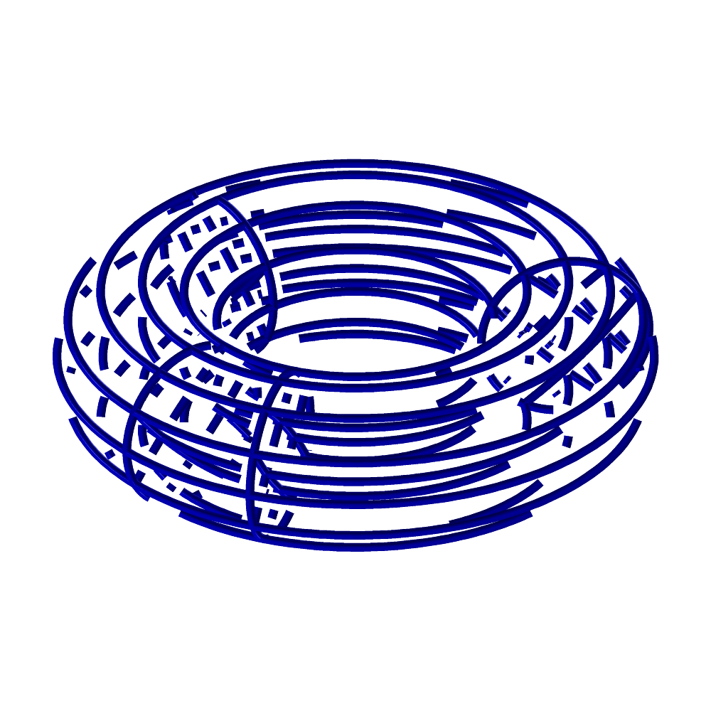
FIGURE:
A trivariate of revolution in the shape of a torus is creating,
using TVREV, by rotating a disk surface.
TVREV2
TrivarType TVREV2( SurfaceType Srf,
NumericType StartAngle,
NumericType EndAngle )
or
TrivarType TVREV2( ListType SrfList,
NumericType StartAngle,
NumericType EndAngle )
computes trivariate(s) of revolution for the given surface(s) by rotating
the input along the Z axis.
Example:
Tv = TVRev( Disk, 90, 270 );
Createa a 1/2 of a trivariate torus, TV by rotating the input Disk
surface along the Z axis.
See also SURFREV, TVPREV, TVREV, TVPREV2.
TVS2FILLET
TrivarType TVS2FILLET( SurfaceType Srf1, SurfaceType Srf2,
NumericType RailDist, NumericType R1Orient,
NumericType R2Orient, NumericType TanScale,
NumericType CtlPts, NumericType Tol,
NumericType NumerTol, NumericType FilletingMethod)
Constructs a (list of) fillet trivariate(s) between Srf1 and
Srf2. The fillet meets with Srf1 and Srf2 with G1
continuity, and its bounded in between their intersection curve and
two rail curves, that are computed as an approximate Euclidean offset
of the intersection curve on each of the surfaces. R1Orient
and R2Orient specify the orientations of the two rail curves
((+/-)1), or can be set to zero to choose the orientation resulting
with the maximal arc length rail curve. TanScale specifies the
magnitude of the fillet's tangets that connect it with Srf1 and
Srf2. CtlPts controls the number of control points used
to approximate some of the curves computed during the filleting
algorithm. Tol and NumerTol specify the tolerances used during the
filleting algorithm. FilletingMethod specifies the used
filleting method (0 for the ruled volume method and 1 for the
volumetric boolean sum method).
Example:
TeapotOrig = load( "teapot" );
Body = nth( TeapotOrig, 1 );
Spout = nth( TeapotOrig, 2 );
filletTV = TVS2FILLET( Body, Spout, 0.3, 1, -1, 0.25, 20,
5e-2, 1e-10, 0);
See also VMDLFILLET, MDLFILLET, TVTTFILLET.
TVTTFILLET
TrivarType TVTTFILLET( TrivarType TV1, TrivarType TV2,
NumericType Bndry1, NumericType Bndry2,
NumericType RailDist, NumericType R1Orient,
NumericType R2Orient, NumericType TanScale,
NumericType CtlPts, NumericType Tol,
NumericType NumerTol, NumericType FilletingMethod)
Constructs a (list of) fillet trivariate(s) between the specified
boundary surfaces of TV1 and TV2. The fillet meets with
the boundary surfaces with G1 continuity, and its bounded in between
their intersection curve, and two rail curves, that are computed as
an approximate Euclidean offest of the intersection curve on each of
the surfaces. Bndry1 and Bndry2 specify the boundary surfaces of
TV1 and TV2 to construct a fillet in between (0,1,2,3,4,5
for UMin, UMax, VMin, VMax, WMin and WMax, respectively, and 6 to
take a list of all six boundary surfaces). R1Orient and R2Orient} specify the orientations of the two rail curves ((+/-)1),
or can be set to zero to choose the orientation resulting with the
maximal arc length rail curve. TanScale specifies the
magnitude of the fillet's tangets that connect it with TV1 and
TV2. CtlPts controls the number of control points used
to approximate some of the curves computed during the filleting
algorithm. Tol and NumerTol specify the tolerances used
during the filleting algorithm. FilletingMethod specifies the
used filleting method (0 for the ruled volume method and 1 for the
volumetric boolean sum method).
Example:
Teapot = load( "vteapot2htr_tvs" );
VBody = nth( Teapot, 1 );
VSpout = nth( Teapot, 3 );
filletTV = TVTTFILLET( VBody, VSpout, 5, 5, 0.3, 1, -1, 0.25, 20,
5e-2, 1e-10, 0);
See also VMDLFILLET, MDLFILLET, TVS2FILLET.
TVZRJACOB
PolyType TVZRJACOB( TrivarType TV,
NumericType Euclidean,
NumericType SkipRate,
NumericType Fineness )
computes the zero set of the Jacobian of the given trivariate, TV.
This zero set is the implicit boundary of the trivariate and, for example,
equals the envelop of the sweep of a bivariate surface in space (see
example below). The zero set is returned as a polygonal data set
approximation with Fineness tolerance. If Euclidean, the
resulting polygons are in Euclidean space. Otherwise, the polygons are
returned in the trivariate's parametric domain. Finally, SkipRate
provides a mechanism to skip to every SkipRate row, column and plane
while a SkipRate skips nothing.
Example:
Tv = tfromsrfs( list( Srf,
Srf * tx( 3 ) * ty( 3 ),
Srf * tx( 6 ) ), 3 );
Tv1ZeroJacobian = TVZRJACOB( Tv, 1, 1, 0 );
A trivariate TV is constructed as a sweep of surface Srf
along a quadratic Bezier curve with (0, 0), (3, 3), (6, 0) as control points,
and then the zero set of the Jacobian is derived to yield the envelope of
this motion of Srf.
See figure for an example.
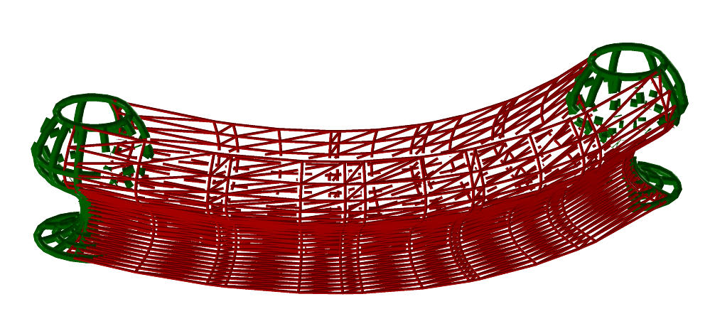
FIGURE:
The envelope of the motion of the wine glass surface in space can
be derived with the aid of the TvZrJacob function.
See also TVJACOBIAN and TVIMPJACOB.
UNITETEXTURE
AnyType UNITETEXTURE( AnyType Geom, StringType MergedTextureName )
Given a model Geom with entries with attribute texture maps,
merges all images into one large image called
MergedTextureName while updating the relative location in
the merged image of each specific texture in each entry.
Example:
MergedTextureModel = UNITETEXTURE( Model, Mergedtexture.png" );
UNSTRCTGRID
CurveType UNSTRCTGRID( NumericType Operation,
ListType Params )
Topological computations over an unstructured grid of points.
Operation can be one of:
0 - create a Params: contains no items. Returns the
new UG. ID of the newly created UG.
1 - free a UG. Params: ID of the UG to free. Returns
Success-flag, i.e., TRUE if successful,
FALSE otherwise.
2 - sets points Params: ID of UG, List of Pts, List of
of a UG. Pt-IDs. Returns Success-flag, vector of
actual IDs assigned to pts in grid.
3 - adds points Params: ID of UG, List of Pts, List of Pt-IDs.
to a UG. Returns Success-flag, ID of new UG, number of
points in grid, vector of actual IDs assigned
to pts in grid.
4 - extract points Params: ID of UG, attribute-type,
with given attribute-names, attribute-values.
attribute values. Returns binary vector with 1s' for selected points.
5 - merge identical Params: ID of UG, flag to identify points
points. without merging, binary vector with 1s' for points
to consider for merge. Returns Success-flag, ID of
new UG, number of points in new UG, vector
indicating which points were identified.
6 - modify a point Params: ID of UG, ID of Point to modify, new
in a UG. coordinates of point. Returns Success-flag.
7 - add a cell Params: ID of UG, Cell, List of point IDs.
to a UG. Returns Success-flag, ID of Cell.
8 - append two UGs. Params: ID of the two UGs to append.
Returns Success-flag, ID of newly created UG,
number of points in new UG, newly assigned IDs
to points in second UG.
9 - update Params: ID of the UG, Tolerance for merging
adjacency relations identical entities. Returns Success-flag.
amongst cells of UG.
10 - purge Params: ID of the UG. Returns Success-flag,
points of UG which ID of new UG, number of points in new UG.
do not belong to
any cell.
11 - ID to Params: ID of UG, ID of Cell.
cell map. Returns Success-flag, Cell.
12 - cell Params: ID of UG, Cell.
to ID map. Returns Success-flag, ID of Cell.
13 - No Support. Params: Contains no item.
14 - No Support. Params: Contains no item.
15 - Extract info Params: ID of UG. Returns Success-flag,
on the UG. Number of points, number of cells, number of
curve cells, number of surface cells, number of
trivar cells, number of cell attributes, number
of points attributes.
16 - Extract the Params: ID of UG. Returns Success-flag,
boundaries of all ID of new UG (extrnal bndry), ID of new UG
curve-cells. (internal bndry), ID of new UG (internal bndry,
different function spaces), number of pts in grid.
17 - Extract the Params: ID of UG. Returns Success-flag, ID
boundaries of all of new UG (extrnal bndry), ID of new UG (internal
surface-cells. bndry), ID of new UG (internal bndry, different
function spaces), number of pts in grid.
18 - Extract the Params: ID of UG. Returns Success-flag, ID
boundaries of all of new UG (extrnal bndry), ID of new UG (internal
trivariate-cells. bndry), ID of new UG (internal bndry, different
function spaces), number of pts in grid.
19 - Set Params: ID of UG, attribute-type, attribute
attributes of name, list of point-ids, list of attribute values.
points. Returns Success-flag.
20 - Get Params: ID of UG, attribute-type, attribute
attributes of name, list of point-ids. Returns Success-flag,
points. list of attribute values.
21 - Set Params: ID of UG, attribute-type, attribute
attributes name, list of cell-ids, list of attribute values.
of cells. Returns Success-flag.
22 - Get Params: ID of UG, attribute-type, attribute
attributes name, list of cell-ids. Returns Success-flag,
of cells. list of attribute values.
23 - Get Params: ID of UG, ID of cell. Returns
adjacency list Success-flag, list of cell-ids adjacent to
for a cell. given cell.
24 - Get list Params: ID of UG. Returns Success-flag,
of point-IDs list of point-IDs, list of cell-IDs of UG.
and cell-IDs.
25 - Get list Params: ID of UG, ID of Cell. Returns
of point-IDs Success-flag, cell type (curve/surface/etc.),
of a cell. list of point-IDs of the cell.
26 - Get list Params: ID of UG. Returns Success-flag,
of all points in UG number of points in the list, the list of IDs,
(including IDs) and a list XYZ points.
27 - Assign ID of new UG, number of points in new UG.
sequential IDs to
points, starting
with 1.
28 - Assign Params: ID of UG. Returns Success-flag,
sequential IDs to ID of new UG, number of points in new UG.
cells, starting
with 1.
29 - Add Params: ID of UG, Object to add.
object to field. Returns Success-flag.
30 - Get Params: ID of UG. Returns
field. Success-flag, field as an object-list.
31 - Add Params: ID of UG, cell to add.
a new cell to Returns Success-flag, number of points in UG.
grid. Also adds
points of cell
to grid.
32 - Extract Params: ID of UG. Returns Success-flag,
Bezier patches of ID of new UG, number of points in new UG.
input UG as a new, Converts all B-spline patches to Bezier.
Bezier's only, UG.
33 - Refine Params: ID of UG, Cell-Id to refine,
cells. direction to refine, parameter values to refine
at, number of values. Returns Success-flag,
ID of new UG, number of points in new UG.
34 - Select Params: ID of UG, point, Closest Entity
cell clostest to (closest face for 1, closest edge for 2, and
given point. closest corner for 2). Optionally, can have
a fourth parameter with an attribute to place
on the selected entity, as
"list( attrName, AttrVal )".
Returns Success-flag, ID of selected cell,
selected face and selected edge.
35 - Select Params: ID of UG, polyline, direction.
all cells Returns Success-flag, IDs of cells selected,
intersecting with number of cell IDs.
frustum of given
polyline and vector.
36 - Refine Params: ID of UG, RefRatio, Pt, Div1
cells at Point. Div2, Div3. Div1/2/3 refer to divisions to
refine at for closest entity to Pt. Div1 must
be positive. If Div2 < 0, closest edge is
considered and refined Div1 times. If Div2 > 0
and Div3 < 0, closest face is considered and
refined Div1 x Div2 times. If Div2 > 0
and Div3 > 0, closest volume (trivariate) is
considered and refined Div1 x Div2 x Div3 times.
RefRatio sets the size ratios between the first
division and last (one for similar sizes).
Returns Success-flag, ID of new UG, number
of points in new UG, Cell Id.
37 - Refine Params: ID of UG, RefSize. Refines
unrefined cells. all cells that were unrefined so far in all
dirs., so that all edge lengths in all such
cells are approximately smaller than RefSize.
if RefSize is zero, 5% of the bbox of the
input geometry is set to RefSize. If RefSize
is negative, -Refsize of the bbox of the input
geometry will be used as RefSize.
38 - Write Params: ID of UG, file-name (zero
grid to a file. length name for stdout).
Returns Success-flag.
39 - Read Params: File-name to read from.
grid from disk. Returns Success-flag, ID of new UG, number
of points in new UG.
40 - Converts Params: File-name to read from.
all patches Returns Success-flag, ID of new UG, number
to linear in of points in new UG. Converts all patches
all dimension. to linear Bezier patches. An
approximation of the input UG patches.
Example:
PtList1 = list(
Point(0,0,0), Point(0,0,0), Point(0,1,0), Point(1,1,0),
Point(0,0,1), Point(1,0,1), Point(0,1,1), Point(1,1,1),
Point(0,0,2), Point(1,0,2), Point(0,1,2), Point(1,1,2));
IdList1 = list( 1, 2, 3, 4, 5, 6, 7, 8, 9, 10, 11, 12);
ParList = list ( UG1, PtList1, IdList1);
RetVal = UNSTRCTGRID( UG_SET_POINTS, ParList );
Success = nth( RetVal, 1);
printf( "Set points in grid. Success = %d.\n", list( Success ) );
Creates a UG with 12 points.
UNTRIM
ListType UNTRIM( TrimSrfType TrimSrf, ListType Params, NumericType Compose )
or
ListType UNTRIM( ListType TrimSrfList, ListType Params, NumericType Compose )
Untrims a trimmed surface or a list of trimmed surfaces. The trimmed
surface(s) is/are converted into a set of tensor-product surface
patches by tiling its valid (untrimmed) parametric domain with
parametric tensor product quads only to compose the parametric quads
with the input (tensor product) surface(s).
The untrimming is performed by the line-sweep algorithm (if Params
is an empty list), or by the minimum-weight algorithm with either a
pre-defined weight function below (if Params contains a single
value) between 1 to 3, or a weight blend of the three weight
functions below (if Params contains a list of three real values,
indicating weights). The pre-defined weight function are:
1. A function which favors a low ratio between the maximum Jacobian
determinant of the surface patches and the minimum Jacobian
determinant (in absolute values).
2. A function which favors close-to-orthogonal isoparametric curves
in the surface patches.
3. A function which favors surface patches which are close to being
square (i.e. height similar to width) in the parametric domain of
the input surface.
If Compose is true, the resulting untrimmed surface patches
will be returned in Euclidean space. Otherwise, they will be returned
in the parametric space of the input surface(s).
Example:
UntrimmedSrfs = UNTRIM( TrimSrf, list(1), true );
See also UNTRIMMED_TYPE.
UVPOLY
PolyType UVPOLY( PolyType Obj, ListType Scales, ListType Translates );
Sets UV coordinates to polygonal object Obj. The UV coordinates
are set using the XY Euclidean coordinates if Scales is a list that
holds two scaling factors (XScale, YScale), or the UV coordinates are
set via the two largest span in XYZ for each polygon, if Scales is
a list of three scaling factors (XScale, YScale, ZScale).
Translates offers a way to shift the UV coordinates in the texture
2D domain, Translates of (0, 0) does nothing.
Needless to say, the ?Scale factors scales the Euclidean coordinates before
being sets as UV texture coordinates.
Example:
UVCube = UVPOLY( Cube, list( 1, 1, 1 ), list( 0, 0 ) );
sets UV coordinates to the six faces of the cube, each face with UV
values between zero and one.
VMBLENDPLN
VMBLENDPLN( VModelType Object, StringType Name, NumericType ZLevel,
ListType NumericValues )
Provides a mechanism to blend property functions of any type at all the
points at height ZLevel associated to a volumetric Object. The
output of the blending process is saved in a '.ppm' file with resolution
NumericValues (0, 1), in a file name provided by Name.
The standard behavior of this function blends the rgb attribute associated
to Object. This behavior can only be modified, providing a user-defined
field function, in C code level, of IRIT.
For example,
s1 = Sphere( Vector( 0, 0, 0 ), 1 );
attrib( s1, "rgb", "255,0,0" );
s2 = Sphere( Vector( 1.5, 0, 0 ), 1 );
attrib( s2, "rgb", "0,255,0" );
obj = s1 + s2;
VMBLENDPLN(obj, "blend.ppm", LIST( 1000, 1000 ) );
blends the RGB color values associated to the spheres s1 and s2 in their
intersection region, saving the output in blend.ppm.
See also ATTRIB for setting attributes, VMBLENDPT for blending the attributes
in a specific (Euclidean) point and VMENCFIELD, for encoding fields.
VMBLENDPT
VMBLENDPT( VModelType Object, ConstantType Oper, PointType Point )
provides a mechanism to blend property functions of any type at point
Point associated to a volumetric Object. The output of the
blending process is a control point holding the values of the property at
the point.
The input parameter Oper controls the different stage of the
blending. A value of 0 indicates initialization, where various quantities
are initialized for fast access; a value of 1 outputs the blend at Point
while a value of 9 frees the auxiliary structures created with the
initialization. The value of the input parameter Point is influential
one for Oper is 1. The standard behavior of this function blends the
rgb attribute associated to Object. In order to modify this behavior, a
different, C code based user-defined function must be provided in C code
level of IRIT.
For example,
s1 = Sphere( Vector( 0, 0, 0 ), 1 );
attrib( s1, "rgb", "255,0,0" );
s2 = Sphere( Vector( 1.5, 0, 0 ), 1 );
attrib( s2, "rgb", "0,255,0" );
obj = s1 + s2;
VMBlendPt(obj, 0, POINT(0, 0, 0)); # init cache
VMBlendPt(obj, 1, POINT(0, 0, 0)); # Evalaute value at given
VMBlendPt(obj, 1, POINT(0.75, 0, 0)); # Euclidean locations.
VMBlendPt(obj, 1, POINT(1.5, 0, 0));
VMBlendPt(obj, 9, POINT(0, 0, 0)); # free cache
blends the RGB color values associated to the spheres s1 and
s2 in (0, 0, 0), (0.75, 0, 0) and (1.5, 0, 0) (Euclidean space coordinates).
See also ATTRIB for setting attributes, VMBLENDPLN for blending the
attributes corresponding to a grid of points for the same height coordinate
and VMENCFIELD, for encoding fields.
VMDLFILLET
VModelType VMDLFILLET( TrivarType TV1, TrivarType TV2,
NumericType Bndry1, NumericType Bndry2,
NumericType RailDist, NumericType R1Orient,
NumericType R2Orient, NumericType TanScale,
NumericType CtlPts, NumericType Tol,
NumericType NumerTol, NumericType FilletingMethod)
Constructs a V-rep model containing a (list of) fillet
trivariate(s) that fill the space between the specified boundary
surfaces of TV1 and TV2. The fillet meets with the
boundary surfaces with G1 continuity, and its bounded in between
their intersection curve and two rail curves, that are computed as an
approximate Euclidean offest of the intersection curve on each of the
surfaces. Bndry1 and Bndry2 specify the boundary
surfaces of TV1 and TV2 to construct a fillet in between
(0,1,2,3,4,5 for UMin, UMax, VMin, VMax, WMin and WMax, respectively,
and 6 to take a list of all six boundary surfaces). R1Orient
and R2Orient specify the orientations of the two rail curves
((+/-)1), or can be set to zero to choose the orientation resulting
with the maximal arc length rail curve. TanScale specifies the
magnitude of the fillet's tangets that connect it with Srf1 and Srf2.
CtlPts controls the number of control points used to approximate
some of the curves computed during the filleting algorithm. Tol and
NumerTol specify the tolerances used during the filleting algorithm.
FilletingMethod specifies the used filleting method (0 for the ruled
volume method and 1 for the volumetric boolean sum method).
Example:
Teapot = load( "vteapot2htr_tvs" );
VBody = nth( Teapot, 1 );
VSpout = nth( Teapot, 3 );
filletVMdl = VMDLFILLET( VBody, VSpout, 5, 5, 0.3, 1, -1, 0.25, 20,
5e-2, 1e-10, 0 );
See also MDLFILLET, TVS2FILLET, TVTTFILLET.
VMDLREV
VModelType VMDLREV( TrimSrfType TSrf, PointType AxisPt, VectorType AxisVec,
NumericType StartAngle, NumericType EndAngle,
NumericType Rational )
or
VModelType VMDLREV( ListType TSrfList, PointType AxisPt, VectorType AxisVec,
NumericType StartAngle, NumericType EndAngle,
NumericType Rational )
constructs a VMODEL out of a given trimmed surface TSrf or trimmed
surfacesTSrfList, by rotating the trimmed surface into a volume of
revolution. AxisPt and AxisVec sets the rotational axis, whereas
StartAngle and EndAngle controls the rotational span. Finally,
Rational controls if the result is a precise (Rational) volume of
revolution, or a polynomial approximation (if input surfaces are polynomial).
Example:
VMRev = VMDLREV( TSrf, point( 0, 0, 0 ), vector( 0, 0, 1 ), 0, 90, false );
constructs a 90 degrees trimmed volume (VMODEL) of revolution around the Z
axis, using TSrf.
See also RULEDVMDL and VMDLSWP, and SURFPREV, SURFPREV2, and SURFREV.
VMDLSWP
VModelType VMDLSWP( TrimSrfType CrossSection, CurveType Axis,
NumericType Scale | CurveType ScaleCrv,
CurveType FrameCrv | VectorType FrameVec | ConstType OFF,
NumericType AxisRefine )
constructs a generalized cylinder VMODEL. This function sweeps a specified
cross section CrossSection along the provided Axis.
The cross section may be scaled by a constant value Scale, or scaled
along the Axis parametric direction via a scaling curve ScaleCrv.
By default, when frame specification is OFF, the orientation
of the cross section is computed using the Axis curve tangent and
normal. However, unlike the Frenet frame, attempt is made to minimize
the normal change, as can happen along inflection points in Axis.
If a VectorType FrameVec is provided as a frame orientation setting,
it is used to fix the binormal direction to this value. In other words, the
orientation frame has a fixed binormal. If FrameVec has an "init"
attribute with a 1 (TRUE) value, this vector is only used as an initial
vector for the first frame.
If a CurveType FrameCrv is specified as a frame orientation
setting, this vector field curve is evaluated at each placement of
the cross section to yield the needed binormal.
AxisRefine an integer value to define possible refinement of the
Axis to better reflect the information in ScalingCrv and the
orientation. A value of zero will force no refinement while a value of
n > 0 will insert n times the number of control points in ScaleCrv
into Axis, better emulating the requested sweep.
If AxisRefine is negative, it is used as a positive value while a
bound on the sweep approximation error is computed and placed as "SweepError"
attribute on the result.
The resulting sweep is only an approximation of the real sweep. The
scaling and axis placement will not be exact, in general.
Manual refinement (in addition to AxisRefine) of the axis curve at
the proper location, where accuracy is important, should improve the accuracy
of the output. The parametric domains of ScaleCrv and FrameCrv do
not have to match the parametric domain of Axis, and their domains are
made compatible by this function.
Example:
VMSwp = vmdlswp( TrimSrf, Axis, SclCrv, vector( 0, 0, 1 ), 0 );
constructs a sweep trimmed volume (VMODEL) along Axis curve,
using TrimSrf. The cross section TrimSrf is scaled along the
Axis by SclCrv and the orientation is fixed so the binormal is
the Z axis. No additional refinements are applied.
See also RULEDVMDL and VMDLREV, and SWEEPSRF and SWEEPTV.
VMENCFIELD
VMENCFIELD( VModelType Object, StringType String, ConstantType Samples,
ConstantType Output )
provides a mechanism to encode a (scalar, vector, etc.) field String
defined over the V-model Object into a set of property functions associated
to the single V-primitives through least mean square approximation.
The input parameter Samples controls the number of evaluated points
for each knot span of each trivariate B-spline, so as to guarantee the
Schoenberg-Whitney interpolation conditions. The value Output controls
the output of the method: TRUE if the output property functions are to be
returned as a separate trivariate structure and FALSE if they are to be
encoded in the same trivariates describing the geometry of Object.
The standard behavior of this function blends the rgb attribute
associated to Object. In order to modify this behavior, a different,
user-defined function must be provided directly in C code level of IRIT.
For example,
s1 = Sphere( Vector( 0, 0, 0 ), 1 );
attrib( s1, "rgb", "255,0,0" );
s2 = Sphere( Vector( 1.5, 0, 0), 1 );
Attrib( s2, "rgb", "0,255,0" );
obj = s1 + s2;
objRec = VMENCFIELD( obj, "", FALSE );
SAVE("output1", objRec);
encodes the RGB color values given as attributes to s1 and s2 into the
V-model objRec and save the new V-model into a itd file.
See also ATTRIB for setting attributes, VMBLENDPLN and VMENCFIELD.
VMSLICE
AnyType VMSLICE( TrivarType Model | VModelType Model,
NumericType SliceMode,
StringType SliceImageName,
VectorType ZLevels,
ListType Options );
Given a volumetric object, Model, either a TRIVAR, a list of
TRIVARs. or a VMODEL model, slice it at level ZLevel, or at
levels (Zmin, ZMin, ZStep), from ZMin to ZMax, in ZSteps if
ZLevels.
Options is a list object holding slicing information as
1. If Model is a single trivariate, Options will be
({Mdl,} XMin, YMin, XMax, YMax, ZRes, XRes, YRes)
where Mdl is an optional POLYgonal/MODEL object
setting the boundaries of the sliced volume (i.e. trimming
boundaries of the trivar).
If a non zero interger attribute named "level" is detected
in Mdl, the whole VMSLICE processing will be
restricted to the interior of Mdl.
The rest of the parameters set the XY domain to slice and the
resolution.
2. If Model is a list of more than one trivariate, Options
will be
({Mdl,} XMin, YMin, XMax, YMax, ZRes, XRes, YRes)
where Mdl is an optional containter holding all
trivariates in the list. Mdl in this case, can be one
of a TRIVAR, a MODEL, a VMODEL, or a POLYgonal model.
This optional container can serve as a (transparent)
aquarium to hold all the content. The color and
transparency attributes of this container are employed.
If a non zero interger attribute named "level" is detected
in Mdl, the whole VMSLICE processing will be
restricted to the interior of Mdl.
The rest of the parameters set the XY domain to slice and
the resolution.
3. If Model is a a VMODEL, Options will be
(Idx, XMin, YMin, XMax, YMax, ZRes, XRes, YRes)
where Idx sets the index of the VElement in the VMODEL to
slice. If Idx is negative, all the VMODEL is sliced.
The rest of the parameters set the XY domain to slice and the
resolution.
If the optional POLYgonal/MODEL, {Mdl}, as first parameter of the
Options is provided and Mdl has both "rgb" and "transp", then
it will be scan converted into the slices as well, in pixels that are
not affected by Model. Otherwise, it will only serve to
restrict Model to its volume.
All dimensions are in Object space resolution. SliceMode can be
0. Slice a heterogenenous image.
1. Slice and return the outline curves of the intersection as
curves.
2. Slice and return the outline curves as an image.
3. Slice and return the full covering set as linear curves.
4. Slice and return the full covering set as an image.
Example:
vmslice( TV, 0, "vmslice.ppm", 1.0,
list( Mdl, 0.0, 0.0, 1.0, 1.0, 0.01, 0.01, 0.01 ) );
slices heterogeneous (E4, E6, etc.) trivariate TV in domain
[0, 1]^2 in XY and resolution 0.01, into image vmslice.ppm.
See also MICROSLICE
VOXELIZE
VoxelType VOXELIZE( CurveType Crv | ModelType Mdl || TrivarType TV |
VModelType VMdl | ListType Lst,
NumericType PixelType, ListType Resolution );
Given (closed) geomerty, as curve Crv, trivariate TV, model
Mdl, or vmodel Vmdl or a list of such geometries Lst,
convert the given geometry into voxels model at the designated Resolution} that is a list of resolution in X, Y, and Z. Returned is
vxls model. The pixel type in the create voxel model can be one of
1 (unsigned byte), 2 (int), 3 (double), 4 (ARGB byte), 5 (ARGB int),
6 (ARGB double), where ARGB stands for 4 entities: Alpha, Red, Green,
and Blue.
Example:
vxls = voxelize( tv, list( 1, 0.1, 0.1, 0.1 ) );
See also OFFSET that con computes offsets over voxels, and VOXELOPER for
special voxels operations.
VOXELOPER
AnylType VOXELOPER( VoxelType VxlMdl, NumericType Operation,
NumericType OperValue );
or
AnylType VOXELOPER( VoxelType VxlMdl, NumericType Operation,
ListType OperValues );
or
AnylType VOXELOPER( NumericType Dummy, NumericType Operation,
ListType OperValues );
performs operations over a Voxeltype model VxlMdl.
Operations prescribes the operation to perform and OperValue
sets an input value for the operations. Operations Can be one of:
0 with OperValues being a list of two parameters as
(PixelFormat, ImageIdx), prints the Voxel Model to
stderr using pixel format string PixelFormat, and dumps the
ImageIdx image plane in the volume. If ImageIdx is less
than zero, all image planes and hence all volume is dumped to
stderr.
1 Applies marching cubes to VxlMdl, with numeric parameter
iso value OperValue. Result is a polygonal model
representing the iso surface of VxclMdl, at iso level
OperValue.
3 Computes a voxel model using radon transform between n (can be more
than two images!). Herein, VxlModel can be a Dummy
numeric value that is ignored.
Images are given in OperValues as a list of lists, each
sub-list holds two items - image file name (a string) and a
horizontal view angle.
Example:
MCPolys = VoxelOper( vxl, 1, 100 );
See also VOXELIZE that converts geometry into a VoxelType Model.
ZCOLLIDE
NumericType ZCOLLIDE( GeometricTreeType Obj1,
GeometricTreeType Obj2,
NumericType Fineness,
NumericType NumOfIters );
Given two objects, Obj1 and Obj2, where Obj1 is assumed to
be above (in the Z direction) Obj2, this function computes the amount
that Obj1 could be moved down, the -Z direction, until it collides with
Obj2. The collision detection is considered using a polygonal
approximation that has a Fineness resolution (see RESOLUTION variable).
The computation cost is linear in NumOfIters with quadratic accuracy
convergence. Values of ten for both Fineness and NumOfIters are
reasonable selections. While Obj1 is considered in its exact form, in
Obj2, only the bbox of the shape is considered.
Example:
view( chair, 1 );
for ( x = 0, 1, 5,
b = box( vector( x / 10, 0, 2 ), 0.1, 0.1, 0.1 ):
view( b * tz( ZCOLLIDE( chair, b, 10, 10 ) ), 0 ) );
places and draws six different cubes on top of the object called chair.
ZTEXTRUDE
SurfaceType ZTEXTRUDE( CurveType CrossSection, NumericType Rational,
NumericType ZPitch )
or
TrivarType ZTEXTRUDE( SurfaceType CrossSection, NumericType Rational,
NumericType ZPitch )
constructs an extrusion of CrossSection in the +Z direction
while twisting (rotation the CrossSection along the Z axis).
ZPitch sets the Z extrusion amount (for 360 rotation) as we
advances in the +Z direction.
If Rational is TRUE the result is a precise rational freeform. If
FALSE, a polynomial approximation is constructed instead.
Example:
TV = ZTEXTRUDE( Srf, TRUE, 1 );
See figure for an example.
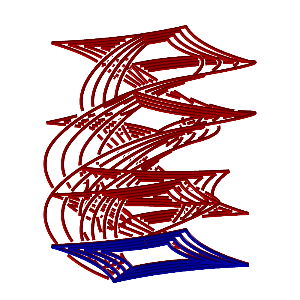
FIGURE:
A twisting extrusion can be constructed via the ZTEXTRUDE command.
Here a start shaped planar surface ( in blue) is extruded and
twisted to created the shown trivariate (in red).
See also EXTRUDE.
Object transformation functions
All the routines in this section construct a 4 by 4 homogeneous
transformation matrix representing the required transform. These matrices
may be concatenated to achieve more complex transforms using the matrix
multiplication operator *. For example, the expression
m = trans( vector( -1, 0, 0 ) ) * rotx( 45 ) * trans( vector( 1, 0, 0 ) );
constructs a transform to rotate an object around the X = 1 line, 45 degrees.
A matrix representing the inverse transformation can be computed as:
InvM = m ^ -1
See also overloading of the - operator.
HOMOMAT
MatrixType HOMOMAT( ListType MatData )
creates an arbitrary homogeneous transformation matrix by manually providing
its 16 coefficients.
Example:
step = 10;
for ( a = 1, 1, 720 / step,
view_mat = save_mat *
HOMOMAT( list( list( 1, 0, 0, 0 ),
list( 0, 1, 0, 0 ),
list( 0, 0, 1, -a * step / 500 ),
list( 0, 0, 0, 1 ) ) ):
view( list( view_mat, axes ), on )
);
looping and viewing through a sequence of perspective transforms, created
using the HOMOMAT constructor. See also RFLCTMAT and PROJMAP.
MAP3PT2EQL
MatrixType MAP3PT2EQL( PointType Pt1, PointType Pt2, PointType Pt3 )
computes the transofrmation matrix in the XY plane that takes the given
three planar points into an equilateral triangle around the origin.
Example:
Mat = MAP3PT2EQL( Pt1, Pt2, Pt3 );
See also ELLIPSE3PT, CONICSEC.
MATPOSDIR
MatrixType MATPOSDIR( PointType Pos, VectorType Dir, VectorType UpDir )
creates a viewing transformation matrix of a viewer at Pos, looking
at direction Dir and upper view of UpDir.
Example:
step = 10;
for ( a = 1, 1, 720 / step,
view_mat = MATPOSDIR( point( 0.5, 0.1, 0.5 ),
vector( 0.0, 1.0, 0.0 ),
vector( cos( a * step * Pi / 360 ), 0,
sin( a * step * Pi / 360 ) ) ):
view( list( view_mat, axes ), on )
);
looping and viewing through a sequence of transforms, created
using the MATPOSDIR constructor.
PROJMAT
MatrixType PROJMAT( PlaneType ProjPlane,
VectorType EyePos,
NumericType EyeInf )
constructs a projection matrix to project the universe onto the given
projection plane ProjPlane, with the eye position at EyePos
(divided by EyeInf). Note that if EyeInf is zero, the eye is
at infinity.
Example:
PMat = PROJMAT( plane( 0, 0, 1, -0.1 ), vector( 1, 1, 1 ), 0 );
contstructs a projection matrix PMat onto the Z = -0.1 plane
with a view direction of ( 1, 1, 1 ). See also RFLCTMAP, HOMOMAT.
PSELFINTER
PolyType PSELFINTER( PolyType PolyObj )
computes theslef intersections, if any, of polygons in PolyObj.
Example:
SelfInters = PSELFINTER( Poly );
PRULEDALG
CurveType PRULEDALG( SurfaceType Srf, NumericType Tolerance,
NumericType Euclidean, NumericType CrvSizeReduction,
NumericType SubdivTol, NumericType NumericTol,
NumericType GenSurfaces )
or
CurveType PRULEDALG( TrimSrfType Srf, NumericType Tolerance,
NumericType Euclidean, NumericType CrvSizeReduction,
NumericType SubdivTol, NumericType NumericTol,
NumericType GenSurfaces )
computes a piecewise ruled surface approximation to given surface Srf,
where the fit always starts from VMin parametric direction.
The strips fits Srf to within Tolerance.
If Euclidean is true, the result is evaluated into Euclidean space,
otherwise it is returned in the parametric domain of Srf.
CrvSizeReduction is used as a curve fitting size limit for the
intermediate rail curves of the fruled fitting.
See MZERO for the meaning of SubdivTol and NumericTol.
If GenSurfaces is true, the urled surfaces are returned. Otherwise,
the adjacent ruling lines, as curves, are returned.
Example:
Strips = PRULEDALG( Srf2, 0.01, true, 40, 0.01, 1e-10 );
See figure for an example.
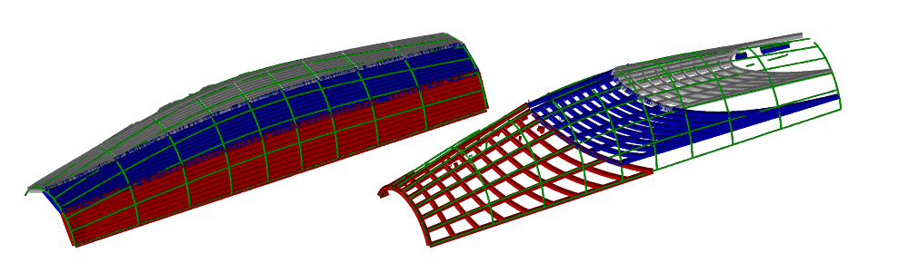
FIGURE:
A ruled surface fitting along two different parametric directions
of the input surface, computed using PRULEDALG.
In blue, the boundaries of the strips are shown while in red, the
tangency curves are presented, between the original surface and the
fitted ruled surface.
See also PRISA and SDVLPCRV.
RFLCTMAT
MatrixType RFLCTMAT( PlaneType RflctPlane )
constructs a reflection matrix to reflect the universe along the given
reflection plane RflctPlane.
Example:
PMat = RFLCTMAT( plane( 0, 0, 1, 0 ) );
constructs a reflection matrix PMat around the Z = 0 plane.
See also PROJMAP, HOMOMAT.
ROTV2V
MatrixType ROTV2V( VectorType Vec1, VectorType Vec2 )
creates a rotation that takes vector Vec1 to vector Vec2.
See also ROTVEC, ROTZ2V, ROTZ2V2.
ROTVEC
MatrixType ROTVEC( VectorType Vec, NumericType Angle )
creates a rotation around the vector Vec matrix with Angle degrees.
See also ROTV2V, ROTZ2V, ROTZ2V2.
ROTX
MatrixType ROTX( NumericType Angle )
creates a rotation around the X transformation matrix with Angle degrees.
ROTY
MatrixType ROTY( NumericType Angle )
creates a rotation around the Y transformation matrix with Angle degrees.
ROTZ
MatrixType ROTZ( NumericType Angle )
creates a rotation around the Z transformation matrix with Angle degrees.
ROTZ2V
MatrixType ROTZ2V( VectorType Dir )
creates a rotation matrix that takes Z axis into Dir. Length of Dir
is ignored.
See also ROTV2V, ROTVEC, ROTZ2V2.
ROTZ2V2
MatrixType ROTZ2V2( VectorType Dir, VectorType Dir2 )
creates a rotation matrix that takes the Z axis into Dir, while the X
axis is aligned with Dir2. The lengths of Dir and Dir2 are
ignored.
See also ROTV2V, ROTVEC, ROTZ2V, ROTVEC.
SCALE
MatrixType SCALE( VectorType ScaleFactors )
creates a scaling by the ScaleFactors transformation matrix.
TRANS
MatrixType TRANS( VectorType TransFactors )
creates a translation by the TransFactors transformation matrix.
General purpose functions
ADWIDTH
ADWIDTH( GeometricType Object, NumericType DWidth )
sets the width of the object. This display width is used in pixels in
display devices for width of line drawing, if supported by the display device.
See also ATTRIB, COLOR, and AWIDTH.
This function is equivalent to using,
ATTRIB( Object, "dwidth", DWidth );
ATTRIB
ATTRIB( AnyType Object, StringType Name, AnyType Value )
provides a mechanism to add an attribute of any type to an Object,
with name Name and value Value. This ATTRIB function is tuned
and optimized toward numeric values or strings as Value although any
other object type can be saved as attribute.
These attributes may be used to pass information to other programs about
this object, and are saved with the objects in data files.
Attributes placed on a list object or even a whole hierarchy of
objects will be propagated into all items in the list or hierarchy.
There are a few exception to this propagation. The "animation" attribute
is not propagated and is kept in the internal nodes, forming a hierachy of
animation commands for all the objects contained in the list/hierarchy.
The "invisible" attribute is saved at all levels of the hierarchy, used to
denote a complete sub tree that is invisible (yet can serve as a source at
which instances can point).
For example,
ATTRIB(Glass, "rgb", "255,0,0");
ATTRIB(Glass, "refract", "1.4");
.
.
.
RmAttr(Glass, "rgb", 0); # Removes "rgb" attribute.
sets the RGB color and refraction index of the Glass object and
later removes the RGB attribute.
Attribute names are case insensitive. Spaces are allowed in the Value
string, as well as the double quote itself, although the latter must be
escaped:
ATTRIB(Glass, "text", "Say "this is me"");
See also RMATTR for removal of attributes, CPATTR for copying them,
GETATTR to get an attribute, ATTRPROP for setting attributes on all
subtrees of parts, as well as AWIDTH, ADWIDTH, FINDATTRm COLOR and PATTRIB.
ATTRPROP
ATTRPROP( AnyType Object, StringType Name, AnyType Value )
Same as ATTRIB but propagates the attributes to all sub-parts of the
object. See also ATTRVPROP.
Example:
Glass1 = list( Base, Handle, Wine );
Glass2 = list( Base, Handle, Wine );
attrib( Glass1, "ptexture", "marble1.gif" );
ATTRPROP( Glass2, "ptexture", "marble1.gif" );
In Glass1, only Glass1 will be set with "texture" while in
Glass2, the "texture" attribute will propagate to the sub-parts of
Glass2, namely to the Base, Handle, Wine.
ATTRVPROP
ATTRVPROP( AnyType Object, StringType Name )
Propagates an Object attribute named Name to the vertices in
Object. Typically for RGB color values.
Example:
Obj2 = ATTRVPROP( Obj, "RGB" );
AWIDTH
AWIDTH( GeometricType Object, NumericType Width )
sets the width of the object to one of those specified below. This width
is used in real object side dimensions in tools such as scan converters and
rendering tools for rendering lines and curves, as well as postscript.
See also ATTRIB, COLOR, and ADWIDTH.
This function is equivalent to using,
ATTRIB( Object, "width", Width );
CHDIR
CHDIR( StringType NewDir )
sets the current working directory to be NewDir.
CLNTCLOSE
CLNTCLOSE( NumericType Handler, NumericType Kill )
closes a communication channel to a client. Handler contains the
index of the communication channel opened via CLNTEXEC. If Kill, the
client is sent an exit request for it to die. Otherwise, the communication
is closed and the client runs standing alone. See also VIEWOBJ, VIEWSET,
CLNTREAD, CLNTWRITE, and CLNTEXEC.
Example:
h2 = clntexec( "nuldrvs -s-" );
.
.
.
CLNTCLOSE( h2,TRUE );
closes the connection to the nuldrvs client, opened via CLNTEXEC.
CLNTWRITE
CLNTWRITE( NumericType Handler, AnyType Object )
writes one object Object to a communication channel of a client.
Handler contains the index of the communication channel opened via
CLNTEXEC. If the Handler equals -1, the regular display device
(forked via, for example, VIEWOBJ command) is used. If Handler equals
CLIENTS_ALL, a broadcast of Object to all clients is performed.
See also VIEWOBJ, VIEWSET, CLNTREAD, CLNTCLOSE, and CLNTEXEC.
Example:
h2 = clntexec( "nuldrvs -s-" );
.
.
CLNTWRITE( h2, Model );
.
.
clntclose( h2,TRUE );
writes the object named Model to client through communication channel h2.
COLOR
COLOR( GeometricType Object, NumericType Color )
sets the color of the object to one of those specified below. Note that an
object has a default color (see irit.cfg file) according to its origin -
loaded with the LOAD command, PRIMITIVE, or a BOOLEAN operation result.
The system internally supports colors (although you may have a B&W
system) and the colors recognized are:
BLACK, BLUE, GREEN, CYAN, RED, MAGENTA, YELLOW, and WHITE.
See the ATTRIB command for more fine control of colors using the RGB
attribute. See also AWIDTH and AWIDTH.
This function is equivalent to using,
ATTRIB( Object, "color", Color );
COMMENT
COMMENT
Two types of comments are allowed:
1. One-line comment: starts anywhere in a line at the '#' character, up to
the end of the line.
2. Block comment: starts at the COMMENT keyword followed by a unique
character (anything but white space), up to the second occurrence of that
character. This is a fast way to comment out large blocks.
Example:
COMMENT
This is a comment
CPATTR
CPATTR( AnyType DestObj, AnyType SrcObj )
copies all attribute from object SrcObj into object DestObj. All
attributes, if any, in DestObj are purged. Needless to say, both objects
must exist at the time of attribute copy.
See also ATTRIB, ATTRPROP, GETATTR, RMATTR.
DITHERIMAGE
DITHERIMAGE( StringType InputImage, StringType DitheredImage,
NumericType DitherMatrixSize, NumericType ErrorDiffusion,
ListType Colors, NumericType DitheringMethod)
dithers, possibly with predefined Colors, an InputImage file.
Result is saved in DitheredImage file. DitherMatrixSize sets
the dithering matrix size that can be 2, 3 or 4. If ErrorDiffusion, an
error diffusion algorithm is applied (Floyd Steinberg). Colors holds a
list of colors as a list of triplet RGB lists, to set the colors to use in the
dithering process, or a non list object for BW dithering.
Finally, DitheringMethod can be one of:
0 Regular Floyd Steinberg including BW if no color.
1 Stucki. Subjectively, this look best.
2 Another variation of Floyd Steinberg.
3 Jarvis, Judice, and Ninke.
4 Burkes.
5/6/7 Three variances of Frankie Sierra.
Example:
DITHERIMAGE( "BenGurion.ppm", "BenGurionDither.ppm", 1, true,
list( list( 0, 90, 158 ),
list( 166, 33, 98 ),
list( 200, 189, 3 ),
list( 240, 240, 240 ) ), 0 );
dithers the input image BenGurion.ppm" into "BenGurionDither.ppm"
using four colors.
See figure for an example for BW dithering.
FIGURE:
An examples of dithering an images,
using the DITHERIMAGE function.
See also DITHERWIRE.
ERROR
ERROR( StringType Message);
breaks the execution and returns to the IRIT main loop, after printing a
Message to the screen. This may be useful in user defined functions to
break execution in cases of fatal errors.
EXEC
EXEC( StringType Command );
executes a string Command in the IRIT interepreter, indirectly.
Example:
Univariate2Bezier = function( Polynom, Deg ): x: f:
return = nil():
f = 1:
for ( x = 0, 0.05 / Deg, 1,
EXEC( "f = " + Polynom ):
snoc( ctlpt( E1, f ), return ) ):
return = coerce( cinterp( return, Deg + 1, Deg + 1, PARAM_UNIFORM, FALSE ),
bezier_type );
defines a function that converts univariate expressions into explicit, E1,
Bezier curves. For example
"Univariate2Bezier( "3 * x ^ 2 - 2 * x + 5", 3 );"
would return a cubic Bezier curve representing "3 * x ^ 2 - 2 * x + 5".
EXIT
EXIT()
exits from the solid modeler. NO warning is given!
FOR
FOR( NumericType Start, NumericType Increment, NumericType End, AnyType Body )
executes the Body (see below), while the FOR loop conditions hold.
Start, Increment, End are evaluated first, and the loop is executed
while <= End if Increment > 0, or while >= End if Increment < 0.
If Start is of the form "Variable = Expression", then that variable is
updated on each iteration, and can be used within the body.
The body may consist of any number of regular commands, separated by
COLONs, including nesting FOR loops to an arbitrary level.
Example:
step = 10;
rotstepx = rotx(step);
FOR ( a = 1, 1, 360 / step,
view_mat = rotstepx * view_mat:
view( list( view_mat, axes ), ON )
);
displays axes with a view direction that is rotated 10 degrees at a
time around the X axis.
HELP
HELP( StringType Subject )
provides help on the specified Subject.
Example:
HELP("");
will list all IRIT help subjects.
FNFREE
FNFREE( StringType UserFuncName )
frees a user defined function named UserFuncName. See also FREE.
FREE
FREE( GeometricType Object )
Because of the usually huge size of geometric objects, this procedure
may be used to free them. Reassigning a value (even of different type)
to a variable automatically releases the old variable's allocated space
as well. See also FNFREE.
FUNCTION
FuncName = FUNCTION(Prm1, Prm2, ... , PrmN):LclVal1:LclVar2: ... :LclVarM:
FuncBody;
defines a function named FuncName with N parameters and M local variables
(N, M >= 0). Here is a (simple) example of a function with no local variables
and a single parameter that computes the square of a number:
sqr = FUNCTION(x):
return = x * x;
Functions can be defined with optional parameters and optional local
variables. A function's body may contain an arbitrary set of expressions
including for/while loops, (user) function calls, or even recursive function
calls, all separated by colons.
The returned value of the function is the value of an automatically defined
local variable named return. The return variable is a regular local variable
within the scope of the function and can be used as any other variable.
If a variable's name is found in neither the local variable list nor
the parameter list, it is searched for in the global variable list (outside
the scope of the function). Binding of names of variables is static as in the
C programming language.
Because binding of variables is performed in execution time, there is a
somewhat less restrictive type checking of parameters of functions that are
invoked within a user's defined function.
A function can invoke itself, i.e., it can be recursive. However, since a
function should be defined when it is called, a dummy function should be
defined before the recursive one is defined:
factorial = function(x):return = x; # Dummy function.
factorial = function(x):
if (x <= 1, return = 1, return = x * factorial(x - 1));
Overloading is valid inside a function as it is outside. For example, for
add = FUNCTION(x, y):
return = x + y;
the following function calls are all valid:
add(1, 2);
add(vector(1,2,3), point(1,2,3));
add(box(vector(-3, -2, -1), 6, 4, 2), box(vector(-4, -3, -2), 2, 2, 4));
Finally, here is a more interesting example that computes an approximation
of the length of a curve, using the sqr function defined above:
distptpt = FUNCTION(pt1, pt2):
return = sqrt(sqr(coord(pt1, 1) - coord(pt2, 1)) +
sqr(coord(pt1, 2) - coord(pt2, 2)) +
sqr(coord(pt1, 3) - coord(pt2, 3)));
crvlength = FUNCTION(crv, n):pd:t:t1:t2:dt:pt1:pt2:i:
return = 0.0:
pd = pdomain(crv):
t1 = nth(pd, 1):
t2 = nth(pd, 2):
dt = (t2 - t1) / n:
pt1 = coerce(ceval(crv, t1), e3):
for (i = 1, 1, n,
pt2 = coerce(ceval(crv, t1 + dt * i), e3):
return = return + distptpt(pt1, pt2):
pt1 = pt2);
Try, for example:
crvlength(circle(vector(0.0, 0.0, 0.0), 1.0), 30) / 2;
crvlength(circle(vector(0.0, 0.0, 0.0), 1.0), 100) / 2;
crvlength(circle(vector(0.0, 0.0, 0.0), 1.0), 300) / 2;
See PROCEDURE and IRITSTATE's "DebugFunc" for more.
IF
IF( NumericType Cond, AnyType TrueBody { , AnyType FalseBody } )
executes TrueBody (a group of regular commands, separated by COLONs -
see FOR loop) if the Cond holds, i.e., it is a numeric value other than
zero, or optionally, if it exists, executes FalseBody. If the Cond
does not hold, i.e., it evaluates to a numeric value equal to zero.
Examples:
IF ( machine == IBMOS2, resolution = 5, resolution = 10 );
IF ( a > b, max = a, max = b );
sets the resolution to 10, unless running on an IBMOS2 system, in which
case the RESOLUTION variable will be set to 5 in the first statement, and
set to max to the maximum of a and b in the second statement.
INCLUDE
INCLUDE( StringType FileName )
executes the script file FileName. Nesting of an include file is allowed
up to 10 levels deep. If an error occurs, all open files in all nested files
are closed and data are waited for at the top level (standard input). Files
are searched for inclusion in the current directory. If not found, and the
inclusion is from a different file at some directory, that directory is
searched as well. Finally, if all the above fails, the directories specified
via the IRIT_INCLUDE environment variable are also searched.
A script file can contain any command the solid modeler supports.
Example:
INCLUDE( "/tmp/general.irt" );
includes the file "/tmp/general.irt". Any inclusion inside general.irt will
search for the included file in the current directory, then in /tmp, and then
in the directories specified via IRIT_INCLUDE.
INSERTPOLY
INSERTPOLY( PolyType Poly, PolyType Polys )
inserts, in place, Poly as a new polygon of object Polys.
After the completion of this function Poly is unmodified but Polys
has a new polygon in it.
Example:
X = poly( list( point( 0, 0, 0 ),
point( 0, 1, 0 ),
point( 1, 1, 0 ),
point( 1, 0, 0 ) ), false );
Y = X * tz( 1 );
INSERTPOLY( Y, X );
At the end of the execution of this sequence of command, X contains
two polygons, one at Z = 0 and one at Z = 1. See also MERGEPOLY, SPLITLST.
INTERACT
INTERACT( GeometryTreeType Object )
This is a user-defined function (see iritinit.irt) that does the
following, in order outlined:
Clear the display device.
Display the given Object.
Pause for a keystroke.
This user-defined function in version 4.0 of IRIT is an
emulation of the INTERACT function that used to exist in previous versions.
Example:
INTERACT( list( view_mat, Axes, Obj ) );
displays and interacts with the object Obj and the predefined object
Axes. VIEW_MAT will be used to set the starting transformation.
See VIEW and VIEWOBJ for more.
IQUERY
IQUERY( NumericType QueryType )
A low level query tool for checking the current state of the IRIT internal
tables. According to the values of QueryType the following is printed
to stdout:
QueryType Printed content
1 All the known functions/user defined functions/constants
and parameters/returned values (if any).
2 All the knwon keywords
LIST
ListType LIST( AnyType Elem1, AnyType Elem2, ... )
constructs an object as a list of several other objects. Only a reference
is made to the Elements, so modifying Elem1 after being included in the list
will affect Elem1 in that list next time list is used!
Each inclusion of an object in a list increases its internal used
reference. The object is freed iff theused reference is zero.
As a result, attempt to delete a variable (using FREE) which is referenced
in a list removes the variable, but the object itself is freed only when the
list is freed.
LOAD
AnyType LOAD( StringType FileName )
loads an object from the given FileName. The object may be any object
defined in the system, including lists, in which the structure is recovered
and reconstructed as well (internal objects are inserted into the global
system object list if they have names). If no file type is provided, ".itd"
is assumed.
This command can also be used to load binary files. ASCII regular data
files usually take longer to load than binary files due to
the required parsing. Binary data files can be loaded directly, like ASCII
files in IRIT, but can only be inspected through IRIT tools such
as dat2irit. A binary data file must have a ".ibd" (IRIT Binary Data) type in
its name.
Compressed files can be loaded if the given file name has a postfix
of ".Z" or .".gz". The gnu utility "gzip" will be invoked via a pipe
for that purpose.
See also IRITSTATE's option "FlatLoad" for optioanl flattening of the object
hierarechy during a load.
LOGFILE
LOGFILE( NumericType Set )
or
LOGFILE( StringType FileName )
If Set is non zero (see TRUE/FALSE and ON/OFF), then everything
printed in the input window will go to the log file specified in the
irit.cfg configuration file. This file will be created the first time
logfile is turned ON. If a string FileName is provided, it will
be used as a log file name from now on. It also closes the current log
file. A "LOGFILE( on );" must be issued after a log file name change.
Example:
LOGFILE( "Data1" );
LOGFILE( on );
printf( "Resolution = %lf\n", list( resolution ) );
LOGFILE( off );
to print the current resolution level into file Data1.
MSLEEP
MSLEEP( NumericType MilliSeconds )
causes the solid modeller to sleep for the prescribed time in milliseconds.
Example:
for ( i = 1, 1, sizeof( crvs ),
c = nth( crvs, i ):
color( c, yellow ):
msleep(20):
viewobj( c )
);
displays an animation sequence and sleeps for 20 milliseconds between
iterations.
NREF
AnyType NREF( ListType ListObject, NumericType Index )
returns a reference to the Index (base count 1) element of the
list ListObject. The reference points to the original object and
hence can be used to modify (add attributes for example) to objects in
lists. Assignment of this reference to a new object would result in a copy
of the object. In contrast, a FREE of a reference to an object would have
an undefined result.
Example:
Lst = list( a, b, c );
attrib( NREF( Lst, 2 ), "NewAttr", on );
adds a new attribute to the second element of Lst. See also NTH.
NRMLCONE
ListType NRMLCONE( SurfaceType Srf )
computes a cone that bounds all normals of surface Srf. A
list of two objects, the axis vector of the cone and the opening radius,
in radians, is returned.
Example:
NCone = NRMLCONE( Srf );
Cn = Cone( vector( 0, 0, 0 ), normalize( nth( NCone, 1 ) ),
nth( NCone, 2 ), 0 ) * tz( 1.0 ) * sc( 0.75 );
computes a normals' cone for surface Srf and builds a real cone following
these limits.
NTH
AnyType NTH( ListType ListObject, NumericType Index )
returns the Index (base count 1) element of the list ListObject.
Example:
Lst = list( a, list( b, c ), d );
Lst2 = NTH( Lst, 2 );
and now Lst2 is equal to 'list( b, c )'. See also NREF.
PAUSE
PAUSE( NumericType Flush )
waits for a keystroke. This is nice to have if a temporary stop in a middle
of an included file (see INCLUDE) is required. If Flush is TRUE, then
the input is first flushed to guarantee that the actual stop will occur.
PRINTF
PRINTF( StringType CtrlStr, ListType Data )
This results in a formatted printing routine, following the concepts of the C
programming language's printf routine. CtrlStr is a string object
for which the following special '%' commands are supported:
%d, %i, %u Prints the numeric object as an integer or unsigned integer.
%o, %x, %X Prints the numeric object as an octal or hexadecimal integer.
%e, %f, %g, Prints the numeric object in several formats of
%E, %F floating point numbers.
%s Prints the string object as a string.
%pe, %pf, %pg Prints the three coordinates of the point object.
%ve, %vf, %vg Prints the three coordinates of the vector object.
%Pe, %Pf, %Pg, Prints the four coordinates of the plane object.
%De, %Df, %Dg, Prints the given object in IRIT's data file format.
All the '%' commands can include any modifier that is valid in the C
programming language PRINTF routine, including l (long), prefix
character(s), size, etc. The point, vector, plane, and object commands
can also be modified in a similar way, to set the format of the
numeric data printed.
Also supported are the newline and tab using the backslash escape
character:
PRINTF("\tThis is the char "\%"\n", nil());
Backslashes should be escaped themselves as can be seen in the above example.
Here are few more examples:
PRINTF("this is a string "%s" and this is an integer %8d.\n",
list("STRING", 1987));
PRINTF("this is a vector [%8.5lvf]\n", list(vector(1,2,3)));
IritState("DumpLevel", 9);
PRINTF("this is a object %8.6lDf...\n", list(axes));
PRINTF("this is a object %10.8lDg...\n", list(axes));
This implementation of PRINTF is somewhat different than the C programming
language's version, because the backslash always escapes the next
character during the processing stage of IRIT's parser. That is, the string
'\tThis is the char "\%"\n'
is actually parsed by the IRIT's parser into
'tThis is the char "%"n'
because this is the way the IRIT parser processes strings. The latter
string is the one that PRINTF actually sees.
See also FPRINTF and FPRINTFILE for ways to redirect PRINTF to a file.
FPRINTF
FPRINTF( NumericType FileNandle, StringType CtrlStr, ListType Data );
Similar to PRINTF, but prints to a file, as set via the FileHandle.
See PRINTF for the formatting options - CtrlStr and Data are
identical as in PRINTF. See PRINTFILE how to open/close a file for
printing to file, and get a FileHandle.
See also PRINTF and FPRINTFILE
FPRINTFILE
NumericType PRINTFILE( StringType FileName | NumericType FileHandle );
Opens a file to write to via FPRINTF, if parameter is a FileName.
Closes a file written to via FPRINTF, if parameter is a FileHandle,
as returned by a previous call to FPRINTFILE to open a file.
Retuns a file handle (non-negative numeric) or -1 if error.
Examples:
File1 = FPrintFile( "test1.txt" );
fprintf( File1, "test1 - 1\n", nil() );
fprintf( File1, "test1 - 2 %d\n", list( File1 ) );
File2 = FPrintFile( "test2.txt" );
fprintf( File2, "test2 - 1\n", nil() );
fprintf( File2, "test2 - 2 %d\n", list( File2 ) );
FPrintFile( File1 );
FPrintFile( File2 );
opens two files and write some text into them, only to close the files.
See also PRINTF and FPRINTF
PROCEDURE
ProcName = PROCEDURE(Prm1, Prm2, ... , PrmN):LclVal1:LclVar2: ... :LclVarM:
ProcBody;
A procedure is a function that does not return a value, and therefore the
returned variable (see FUNCTION) should not be used. A procedure is
identical to a function in every other way. See FUNCTION for more.
RESET
RESET()
clears all variables and initializes the environment to the starting state.
User defined functions, however, are kept intact.
RMATTR
RMATTR( AnyType Object, StringType Name, NumericType Options )
removes attribute named Name from object Object. This function
will have no affect on the Object if the Object has no attribute named
Name.
If Name is a zero length string, all attributes are removed.
Options is a bit mask as follows:
0x01 If Object is a list object, the removal procedure will
recurse over all its elements.
0x02 Removes the attributes also from the geometries in the
Object, like curves or models.
Example:
RmAttr( List, "rgb", 3 );
To remove the "rgb" attribute from all elements in List and all its
geometries. See also ATTRIB, ATTRPROP, GETATTR, CPATTR.
SAVE
SAVE( StringType FileName, AnyType Object )
saves the provided Object in the specified file name FileName.
No extension type is needed (ignored if specified), and ".itd" is supplied
by default. The Object can be any object type, including list, in which
the structure is saved recursively. See also LOAD. If a display device is
actively running at the time SAVE is invoked, its transformation matrix
will be saved with the same name but with extension type of ".imd" instead
of ".itd".
This command can also be used to save binary files. ASCII regular data
files usually take longer to load than binary files due to
the required parsing. Binary data files can be loaded directly like ASCII
files in IRIT, but must be inspected through IRIT tools such
as dat2irit. A binary data file must have a ".ibd" (IRIT Binary Data) type in
its name.
This command can also save geometry in one of the following formats:
IGES file, If the file type is either "igs" or "iges".
STL file, if the file type is "stl". If Object has the int
attribute "RegularTriang" as TRUE, the geometry will be regularized
first (no T junctions). If Object has the int attribute
"MultiObjSplit", the data will be saved in one large STL object in
one file if 0, one STL object per IRIT object in one file if 1, or
in one file per IRIT obejct if 2.
OBJ file. if the file type is "obj".
VRML file. if the file type is "wrl".
CNC Gcode tool path file, if the file type is either "nc" or
"gcode". For this format, only univariate data sets (polylines and
curves) will be processed and saved as 3-axis G code commands.
The following attributes are supported in this mode, if found in
Object:
"NCCommentChar" Holds a string of one character to define the
comment character. If exists a header comment is
dumped as well.
"NCDownPlungeRelFeed" Relative feed rate to plunge down (relative to
"NCFeedRate").
"NCDownPlungeZLevel" Distance, above the plunging destination to move
down in fast g0 motion. Infinity to disable and
plunge in g1 all the way, or zero to plunge fast
in g0 all way.
"NCFeedRate" Feedrate to use. Default is 10 mm per second.
"NCMaxXYBridgeGap" The maximal gap in the XY plane to bridge between
adjacent polylines/curves without retraction.
By default, this value is one mm (0.04inch).
"NCMaxZBridgeGap" The maximal gap in Z to bridge between adjacent
polylines/curves without retraction. By default,
this value is two mm (0.08inch).
"NCRetractZLevel" Set as the Z retraction level above the (bounding
box) of the model. By default, the retration level
will be one inch (25mm) above the bounding box of
the model.
"NCReverseZ" If set to a non negative value, the Z coordinates
are assumed reversed. That is the +Z is down.
By default +Z is assumed up.
"NCUpRetractFast" If TRUE, up retracting will be in fast g0 motion.
Otherwise, if FALSE, g1 will be used.
On some platforms, files will be saved compressed if the given file name
has a postfix of ".Z" or ".gz". The gnu "gzip" utility will be invoked via
a pipe for that purpose.
Example:
SAVE( "oObj1.ibd.Z", Obj1 );
Saves Obj1 in the file Obj1.ibd.Z as compressed binary file.
SETNAME
SETNAME( ListType ListObj, NumericType Index, StringType NewName )
sets the name of a sub object of index Index in list object
ListObj to a new name NewName. The index of the first element is
zero.
Example:
A = list( 1, 2, 3 );
SETNAME( A, 0, "First" );
sets the name of the first element in object A to "First".
While it is not a good idea to modify names of objects in the top level
global space, one can use this function to do exactly that. To rename
the object "Axes" to "XYZ", do:
SETNAME( list( Axes ), 0, "XYZ" );
See also GETNAME.
SNOC
SNOC( AnyType Object, ListType ListObject )
This is similar to the lisp cons operator but puts the new Object in
the end of the list ListObject instead of at the beginning.
Example:
Lst = list( axes );
SNOC( Srf, Lst );
and now Lst is equal to the list 'list( axes, Srf )'.
SYSTEM
SYSTEM( StringType Command )
executes a system command Command. For example,
SYSTEM( "ls -l" );
TIME
TIME( NumericType Reset )
returns the time in seconds from the last time TIME was called with
Reset TRUE. This time is CPU time if such support is available
from the system (times function), and otherwise, is real time (time
function).
The time is automatically reset at the beginning of the execution of this
program.
Example:
Dummy = TIME( TRUE );
.
.
.
TIME( FALSE );
prints the time in seconds between the above two time function calls.
VARLIST
VARLIST( NumericType Verbosity )
lists all the currently defined objects in the system. If Verbosoty
equals 0, only object names are printed. If Verbosoty equals 1, all
object geometry is printed.
VECTOR
VectorType VECTOR( NumericType X, NumericType Y, NumericType Z )
creates a vector type object, using the three provided NumericType scalars.
See also PLANE, POINT.
VERIFYSTATE
VERIFYSTATE( NumericType Action )
auxiliary function to verify the state of the variables in the irit
interpreter as follows:
0. to test if state modified and only report changes to stdout.
1. same as 0 but stop script execution, if state modified.
2. dump to stdout all state.
9. to capture irit state.
so typical use will capture (Action = 9) the state only to verify
it at a later time.
VIEW
VIEW( GeometricTreeType Object, NumericType ClearWindow )
displays the (geometric) object(s) as given in Object.
If ClearWindow is non zero (see TRUE/FALSE and ON/OFF), the window is
first cleared (before drawing the objects).
Example:
VIEW( Axes, FALSE );
displays the predefined object Axes in the viewing window on top of
what is drawn already.
In version 4.0, this function is emulated (see iritinit.irt) using the
VIEWOBJ function. In order to use the current viewing matrix, VIEW_MAT
should be provided as an additional parameter. For example,
VIEW( list( view_mat, Obj ), TRUE );
However, since VIEW is a user defined function, the following will not
use VIEW_MAT as one would expect:
VIEW( view_mat, TRUE );
because VIEW_MAT will be renamed inside the VIEW user defined function to
a local (to the user defined function) variable.
In iritinit.irt one can find several other useful VIEW related functions:
VIEWCLEAR Clears all data displayed on the display device.
VIEWREMOVE Removes the object specified by name from display.
VIEWDISC Disconnects from display device (which is still running)
while allowing IRIT to connect to a new device.
VIEWEXIT Forces the display device to exit.
VIEWSAVE Requests the display device to save transformation matrix.
BEEP An emulation of the BEEP command of versions prior to 4.0.
VIEWSTATE Allows change to the state of the display device.
For the above VIEW related functions, only VIEWREMOVE, VIEWSAVE, and
VIEWSTATE require parameters, which are the file name and view state,
respectively. The view state can be one of several commands. See the
display device section for more.
Examples:
VIEWCLEAR();
VIEW( axes, off );
VIEWSTATE( "DrawSurfaceMesh" );
VIEWSTATE( "DrawStyle" );
VIEWSAVE( "matrix1" );
VIEWREMOVE( "axes" );
VIEWDISC();
VIEWOBJ
VIEWOBJ( GeometricTreeType Object )
displays the (geometric) object(s) as given in Object.
Object may be any GeometricType or a list of other
GeometricTypes nested to an arbitrary level.
Unlike IRIT versions prior to 4.0, VIEW_MAT is not explicitly used
as the transformation matrix. In order to display with a VIEW_MAT view,
VIEW_MAT should be listed as an argument (in that exact name) to
VIEWOBJ. The same is true for the perspective matrix PRSP_MAT.
Example:
VIEWOBJ( list( view_mat, Axes ) );
displays the predefined object Axes in the viewing window using the
viewing matrix VIEW_MAT.
VIEWSET
VIEWSET( NumericType DispHandle )
sets the current display device to be DispHandle. DispHandle is
returned by the CLNTEXEC command. The use of the reserved constant of
CLIENTS_ALL would broadcast the viewing commands to all objects.
Example:
h1 = clntexec( DispDeviceName );
h2 = clntexec( DispDeviceName );
clntwrite( h1, sphere( vector( 0, 0, 0 ), 1 ) );
clntwrite( h2, axes );
pause();
VIEWSET( h1 );
viewclear();
viewobj( list( sphere( vector( 0, 0, 0 ), 1 ), axes ) );
VIEWSET( h2 );
viewclear();
viewobj( list( sphere( vector( 0, 0, 0 ), 1 ), axes ) );
pause();
VIEWSET( CLIENTS_ALL );
viewobj( axes );
pause();
viewexit();
opens two display devices, and displays a unit sphere to the first, and the
axes object, to the second. After a pause, displays both objects on both
display devices, then pauses and exits from both.
See also VIEWOBJ, CLNTEXEC, CLNTCLOSE, CLNTREAD, CLNTWRITE.
WHILE
WHILE( NumericType Cond, AnyType Body )
executes the Body (see below), while the WHILE loop condition
Cond is evaluated into a non zero value. Cond is
evaluated before each iteration.
The body may consist of any number of regular commands, separated by
COLONs, including nesting loops to an arbitrary level.
Example:
deg = 0;
rotstepx = rotx( 10 );
WHILE ( deg < 360,
deg = deg + 10:
view_mat = rotstepx * view_mat:
view( list( view_mat, axes ), ON )
);
displays axes with a view direction that is rotated 10 degrees at a
time around the X axis.
System variables
System variables are predefined objects in the system. Any time IRIT is
executed, these variable are automatically defined and set to values which
are sometimes machine dependent. These are regular objects in any other
sense, including the ability to be deleted or overwritten. One can modify,
delete, or introduce other objects using the iritinit.irt file.
AXES
Predefined polyline object (PolylineType) that describes the XYZ axes.
DRAWCTLPT
Predefined Boolean variable (NumericType) that controls whether curves'
control polygons and surfaces' control meshes are drawn (TRUE) or not
(FALSE). Default is FALSE.
FLAT4PLY
Predefined Boolean object (NumericType) that controls the way almost flat
surface patches are converted to polygons: four polygons (TRUE) or only
two polygons (FALSE). Default value is FALSE.
MACHINE
Predefined numeric object (NumericType) holding the machine type as one of
the following constants: MSDOS, SGI, HP, APOLLO, SUN, UNIX, IBMOS2, WINDOWS,
AMIGA, CYGWIN, MACOSX, and LINUX.
POLY_APPROX_OPT
A variable controlling the algorithm to tesselate surfaces into polygons.
If FALSE, that is, uniform, in parametric space, sampling is used. If TRUE,
maximal deviation between the polygonal approximation and the surface is
used, with distance as prescribed by POLY_APPROX_TOL.
POLY_APPROX_UV
A Boolean predefined variable. If TRUE, UV values of surface polygonal
approximation are placed on the attribute lists of vertices.
POLY_APPROX_TOL
A numeric predefined tesselation control on the distance between the surface
and its polygonal approximation in POLY_APPROX_OPT settings.
POLY_APPROX_TRI
A numeric predefined tesselation control. If TRUE, only triangles are
generated in surface tesselations.
POLY_MERGE_COPLANAR
A numeric predefined surface tesselation control. If TRUE, coplanar
adjacent polygons are merged into one.
PRSP_MAT
Predefined matrix object (MatrixType) to hold the perspective matrix
used/set by VIEW and/or INTERACT commands. See also VIEW_MAT.
RESOLUTION
Predefined numeric object (NumericType) that sets the accuracy of the
polygonal primitive geometric objects and the approximation of curves and
surfaces. It holds the number of divisions into which a circle is divided
(with minimum value of 4). If, for example, RESOLUTION is set to 6, then a
generated CONE will effectively be a six-sided pyramid.
It also controls the fineness of freeform curves and surfaces when they are
approximated as piecewise linear polylines, and the fineness of freeform
surfaces when they are approximated as polygons.
VIEW_MAT
Predefined matrix object (MatrixType) to hold the viewing matrix used/set
by VIEW and/or INTERACT commands. See also PRSP_MAT.
System constants
The following constants are used by the various functions of the system to
signal certain conditions. Internally, they are represented numerically,
although, in general, their exact value is unimportant and may be changed
in future versions. In the rare circumstance that you need to know their
values, simply type the constant as an expression.
Example:
MAGENTA;
AMIGA
A constant designating an AMIGA system, in the MACHINE variable.
APOLLO
A constant designating an APOLLO system, in the MACHINE variable.
BEZIER_TYPE
A constant defining a Bezier freeform geometry.
BLACK
A constant defining a BLACK color.
BLUE
A constant defining a BLUE color.
BSPLINE_TYPE
A constant defining a B-spline freeform geometry.
CLIENTS_ALL
A constant defining a request to address (broadcast to) all clients.
COL
A constant defining the COLumn or U direction of a surface or a
trivariate mesh.
CTLPT_TYPE
A constant defining an object of type control point.
CURVE_TYPE
A constant defining an object of type curve.
CYAN
A constant defining a CYAN color.
CYGWIN
A constant designating an IBM system running under Cygwin, in the MACHINE
variable.
DEBUG_EXE
A constant designating DEBUG (1.0) vs RELEASE (0.0) compilation.
DEPTH
A constant defining the DEPTH direction of a trivariate mesh.
See TBEZIER, TBSPLINE.
E1
A constant defining an E1 (X only coordinate) control point type.
E2
A constant defining an E2 (X and Y coordinates) control point type.
E3
A constant defining an E3 (X, Y and Z coordinates) control point type.
E4
A constant defining an E4 control point type.
E5
A constant defining an E5 control point type.
E6
A constant defining an E6 control point type.
E7
A constant defining an E7 control point type.
E8
A constant defining an E8 control point type.
E9
A constant defining an E9 control point type.
FALSE
A zero constant. May be used as a Boolean operand.
GEOM_CONST
Designates a constant shape.
GEOM_LINEAR
Designates a shape of a (piecewise) linear curve.
GEOM_CIRCULAR
Designates a shape of a circle/arc.
GEOM_PLANAR
Designates a planar shape.
GEOM_SPHERICAL
Designates a spherical shape.
GEOM_SRF_OF_REV
Designates a shape that is (a portion of) a surface of revolution..
GEOM_EXTRUSION
Designates a shape that is an extrusion surface.
GEOM_RULED_SRF
Designates a shape that is a ruled surface.
GEOM_DEVELOP_SRF
Designates a shape that is a ruled surface.
GEOM_SWEEP
Designates a shape that is a sweep surface.
GREEN
A constant defining a GREEN color.
GREGORY_TYPE
A constant defining a Gregory freeform geometry.
HP
A constant designating an HP system, in the MACHINE variable.
IBMOS2
A constant designating an IBM system running under OS2, in the MACHINE
variable.
KV_DISC_OPEN
A constant defining an open end condition with a discontinuous uniformly
spaced knot vector. That is, all interior knots are of multiplicity order -1
and are equally spaced.
KV_FLOAT
A constant defining a floating end condition uniformly spaced knot vector.
KV_OPEN
A constant defining an open end condition uniformly spaced knot vector.
KV_PERIODIC
A constant defining a periodic end condition with a uniformly spaced knot
vector.
LINUX
A constant designating an IBM system running under Linux, in the MACHINE
variable.
LIST_TYPE
A constant defining an object of type list.
MACOSX
A constant designating an IBM system running under Mac OSX, in the MACHINE
variable.
MAGENTA
A constant defining a MAGENTA color.
MATRIX_TYPE
A constant defining an object of type matrix.
MSDOS
A constant designating an MSDOS system, in the MACHINE variable.
MODEL_TYPE
A constant defining an object of type model.
MULTIVAR_TYPE
A constant defining an object of type multivariate function.
NUMERIC_TYPE
A constant defining an object of type numeric.
OFF
Synonym for FALSE.
ON
Synonym for TRUE.
P1
A constant defining a P1 (W and WX coordinates, in that order) rational
control point type.
P2
A constant defining a P2 (W, WX, and WY coordinates, in that order) rational
control point type.
P3
A constant defining a P3 (W, WX, WY, and WZ coordinates, in that order)
rational control point type.
P4
A constant defining a P4 rational control
point type.
P5
A constant defining a P5 rational control
point type.
P6
A constant defining a P6 rational control
point type.
P7
A constant defining a P7 rational control
point type.
P8
A constant defining a P8 rational control
point type.
P9
A constant defining a P9 rational control
point type.
PARAM_CENTRIP
A constant defining a centripetal length parametrization.
PARAM_CHORD
A constant defining a chord length parametrization.
PARAM_NIELFOL
A constant defining a Nielson-Foley parametrization.
PARAM_UNIFORM
A constant defining an uniform parametrization.
PI
The constant of 3.141592...
PLANE_TYPE
A constant defining an object of type plane.
POINT_TYPE
A constant defining an object of type point.
POLY_TYPE
A constant defining an object of type poly.
POWER_TYPE
A constant defining a power basis freeform geometry.
RED
A constant defining a RED color.
ROW
A constant defining the ROW or V direction of a surface or a trivariate mesh.
SGI
A constant designating an SGI system, in the MACHINE variable.
STRING_TYPE
A constant defining an object of type string.
SURFACE_TYPE
A constant defining an object of type surface.
SUN
A constant designating a SUN system, in the MACHINE variable.
TRIMSRF_TYPE
A constant defining an object of type trimmed surface.
TRISRF_TYPE
A constant defining an object of type triangular surface.
TRIVAR_TYPE
A constant defining an object of type trivariate function.
TRUE
A non zero constant. May be used as a Boolean operand.
UNDEF_TYPE
A constant defining an object of no type (yet).
UNIX
A constant designating a generic UNIX system, in the MACHINE variable.
UNTRIMMED_TYPE
A constant defining an untrimmed freeform geometry. See also UNTRIM.
VECTOR_TYPE
A constant defining an object of type vector.
VMODEL_TYPE
A constant defining an object of type volumetric model.
WINDOWS
A constant designating an IBM system running under Windows, in the MACHINE
variable.
WHITE
A constant defining a WHITE color.
YELLOW
A constant defining a YELLOW color.
Animation
The animation tool adds the capability of animating objects using
forward kinematics, exploiting animation curves. Each object has
different attributes, that prescribe its motion, scale, and visibility
as a function of time. Every attribute has a name, which designates
its role. For instance, an attribute animation curve named MOV_X
describes a translation motion along the X axis.
How to create animation curves in IRIT
Let OBJ be an object in IRIT which we want to animate.
Animation curves are either scalar (E1/P1) curves or three-dimensional
(E3/P3) curves with one of the following name prefixes:
MOV_X, MOV_Y, MOV_Z Translation along one axis
MOV_XYZ Arbitrary translation along all three axes
ROT_X, ROT_Y, ROT_Z Rotating around a single axis (degrees)
SCL_X, SCL_Y, SCL_Z Scale along a single axis
SCL Global scale
VISIBLE Visibility
The visibility curve is a scalar curve that enables the display of
the object if the visibility curve is positive at time t and disables
the display (hides) the object if the visibility curve is negative at
time t. A positive visibility value between zero and one also hints at
the opacity of the object, if supported; one means fully opaque.
The animation curves are all attached as an attribute named "animation"
to the object OBJ.
Example:
mov_x = cbezier( list( ctlpt( E1, 0.0 ),
ctlpt( E1, 1.0 ) ) );
scl = cbezier( list( ctlpt( E1, 1.0 ),
ctlpt( E1, 0.1 ) ) );
rot_y = cbezier( list( ctlpt( E1, 0.0 ),
ctlpt( E1, 360.0 ) ) );
attrib(OBJ, "animation", list( mov_x, scl, rot_y ) );
The above will animate OBJ between time zero and one (Bezier curves are always
between zero and one), by moving it a unit size in the X direction,
scaling it to 10% of its original size and rotating it at increasing
angular speed from zero to 360 degrees.
OBJ can now be saved into a file or displayed via one of the regular
viewing commands in IRIT (i.e. VIEWOBJ).
Animation is not always between zero and one. To that end, one can
apply the CREPARAM function to modify the parametric domain of the
animation curve. The convention is that if the time is below the
starting value of the parametric domain, the starting value of the
curve is used. Similarly, if the time is beyond the end of the
parameter domain of the animation curve, the end value of the
animation curve is used.
Example:
CREPARAM( mov_x, 3.0, 5.0 );
to set the time of the motion in the x axis to be from t = 3 to
t = 5. For t < 3, use mov_x(3), and for t > 5, use mov_x(5).
The animation curves are regular objects in the IRIT system. Hence,
only one object named mov_x or scl can exist at one time. If you
create a new object named mov_x, the old one is overwritten! To
preserve old animation curves you can detach the old ones by executing
'free(mov_x)' which will remove the object named mov_x from IRIT's object
list but not from its previously used locations within other list
objects, if any. A different way to do this is to call the animation curves
mov_x1, mov_x2 etc. as only the prefix of the name is verified.
For example:
mov_x = cbezier( list( ctlpt( E1, 0.0 ),
ctlpt( E1, 1.0 ) ) );
attrib(obj1, "animation", list( mov_x ) );
free(mov_x);
mov_x1 = cbezier( list( ctlpt( E1, 2.0 ),
ctlpt( E1, 3.0 ) ) );
mov_x2 = cbezier( list( ctlpt( E1, 2.0 ),
ctlpt( E1, 3.0 ) ) );
attrib(obj2, "animation", list( mov_x1, mov_x2 ) );
free(mov_x);
Notice the way we have two animation curves translating obj2 in x.
This is somewhat artificial but makes more sense if other
transformations appear in between.
One can evaluate an object with animation curves at a certain time, only
to find the proper expected transformation matrix at that time on the
object as an "animation_mat" attribute. The following example defines
a user defined TransformAnim function that creates a transformed
object out of object that was evaluated with ANIMEVAL. Then, a simple loop
(slowly) animates the scene...
TransformAnim = function( Obj ):
return = 0;
TransformAnim = function( Obj ): m: i:
if ( thisobj( "Obj" ) == list_type,
return = nil():
for ( i = 1, 1, sizeof( Obj ),
snoc( TransformAnim( nth( Obj, i ) ), return ) ),
return = Obj * tx( 0 ) ):
m = getattr( Obj, "animation_mat" ):
if ( thisobj( "m" ) == matrix_type,
return = return * m );
for ( t = 0, 0.1, 1,
ANIMEVAL( t, Object ):
view( TransformAnim( Object ), 1 ) );
Animation of movies are supported to a certain extent. A movie animation
is prescribed using a "pmovie" (parametric texture movie) attribute. The
format of the "pmovie" attribute is as follows
"MovieName {, S X Y {Z}} {, F} {, R} {, T=tmin,tmax}"
where "{S} X{,} Y{,} {Z{,}}" prescribes image scaling much like
regular "ptexture" attributes (how many times the image will span the
object?) with the default being for the movie to span the entire
object and 'F' requests the flipping of the X and Y axes of the movie,
again much like in the "ptexture' attribute. Further, "T=tmin,tmax"
sets the time range to execute the animation at, beginning to end and
'R', if set, request that the movie will be repeated modulus this
(tmin,tmax) domain.
A more complete animation example
a = box( vector( 0, 0, 0 ), 1, 1, 1 );
b = box( vector( 0, 0, 0 ), 1, 1, 1 );
c = box( vector( 0, 0, 0 ), 1, 1, 1 );
d = sphere( vector( 0, 0, 0), 0.7 );
pt0 = ctlpt( e1, 0.0 );
pt1 = ctlpt( e1, 1.0 );
pt2 = ctlpt( e1, 2.0 );
pt6 = ctlpt( e1, 6.0 );
pt360 = ctlpt( e1, 360.0 );
pt10 = ctlpt( e1, -4.0 );
pt11 = ctlpt( e1, 1.0 );
pt12 = ctlpt( e1, 4.0 );
pt13 = ctlpt( e1, -1.0 );
visible = creparam( cbezier( list( pt10, pt11 ) ), 0.0, 5.0 );
mov_x = creparam( cbezier( list( pt0, pt6, pt2 ) ), 0.0, 1.2 );
mov_y = mov_x;
mov_z = mov_x;
rot_x = creparam( cbspline( 2,
list( pt0, pt360, pt0 ),
list( KV_OPEN ) ),
1.2, 2.5 );
rot_y = rot_x;
rot_z = rot_x;
scl = creparam( cbezier( list( pt1, pt2, pt1, pt2, pt1 ) ),
2.5, 4.0 );
scl_x = scl;
scl_y = scl;
scl_z = scl;
mov_xyz = creparam( circle( vector( 0, 0, 0 ), 2.0 ), 4.0, 5.0 );
attrib( d, "animation", list( mov_xyz, visible ) );
free( visible );
visible = creparam( cbezier( list( pt12, pt13 ) ), 0.0, 5.0 );
attrib( a, "animation", list( rot_x, mov_x, scl, scl_x, visible ) );
attrib( b, "animation", list( rot_y, mov_y, scl, scl_y, visible ) );
attrib( c, "animation", list( rot_z, mov_z, scl, scl_z, visible ) );
color( a, red );
color( b, green );
color( c, blue );
color( d, cyan );
demo = list( a, b, c, d );
interact( demo );
viewanim( 0, 5, 0.01 );
In this example, we create four objects, three cubes and one sphere.
Animation curves to translate the three cubes along the three axes for
time period of t = 0 to t = 1.2 are created. Rotation curves to
rotate the three cubes along the three axes are then created for time
period t = 1.2 to t = 2.5. Finally, for time period t = 2.5
to t = 4.0. the cubes are (not only) unifomly scaled. For time
period t = 4 to t = 5, the cubes become invisible and the sphere,
which becomes visible, is rotated along a circle of radius 2.
Another complete animation example
This example demonstrates the ability to put "animation" attributes
on internal nodes of a hierarchy, thereb, affecting the entire set of objects
in the hierachy. Herein, we present an robotic arm with three edges
and two joints.
BoxLength = 2;
BoxWidth = 2;
BoxHeight = 10;
LowerBox = box( vector( -BoxLength / 2, -BoxWidth / 2, 0 ),
BoxLength, BoxWidth, BoxHeight);
MiddleBox = box( vector( -BoxLength / 2, -BoxWidth / 2, 0 ),
BoxLength, BoxWidth, BoxHeight);
UpperBox = box( vector( -BoxLength / 2, -BoxWidth / 2, 0 ),
BoxLength, BoxWidth, BoxHeight);
Cn1 = cone( vector( 0, 0, 0 ), vector( 0, BoxHeight / 3, 0 ), 1 );
color( LowerBox, magenta );
color( MiddleBox, yellow );
color( UpperBox, cyan );
color( Cn1, green );
rot_x1 = creparam( cbspline( 3,
list( ctlpt( E1, 0 ),
ctlpt( E1, -200 ),
ctlpt( E1, 200 ),
ctlpt( E1, 0 ) ),
list( KV_OPEN ) ),
0, 3 );
rot_x2 = creparam( cbspline( 4,
list( ctlpt( E1, 0 ),
ctlpt( E1, 400 ),
ctlpt( E1, -400 ),
ctlpt( E1, 0 ) ),
list( KV_OPEN ) ),
0, 3 );
rot_y = creparam( cbspline( 2,
list( ctlpt( E1, 0 ),
ctlpt( E1, 100 ),
ctlpt( E1, -100 ),
ctlpt( E1, 0 ) ),
list( KV_OPEN ) ),
0, 3 );
rot_z = creparam( cbspline( 2,
list( ctlpt( E1, 0 ),
ctlpt( E1, 1440 ) ),
list( KV_OPEN ) ),
0, 3 );
Translate = trans( vector( 0, 0, BoxHeight ) );
attrib( Cn1, "animation", list( rot_z, Translate ) );
Upr = list( Cn1, UpperBox );
attrib( Upr, "animation", list( rot_y, Translate ) );
Mid = list( Upr, MiddleBox );
attrib( Mid, "animation", list( rot_x2, Translate ) );
rbt_hand = list( Mid, LowerBox );
attrib( rbt_hand, "animation", list( rot_x1 ) );
view( rbt_hand, 1 );
In this example, we create four objects, three cubes and one cone,
simulating a robotic hand with three edges an a gripper (the cone).
The animation is defined hierarchically, making it very easy to model
the robot.
Display devices
The following display device drivers are available,
Device Name Invocation Environment
xgldrvs xgldrvs -s- SGI 4D GL regular driver.
xogldrvs xogldrvs -s- SGI 4D Open GL/Motif driver.
xgladap xgladap -s- SGI 4D GL adaptive isocurve
experimental driver.
x11drvs x11drvs -s- X11 driver.
xmtdrvs xmtdrvs -s- X11 Motif driver.
xglmdrvs xglmdrvs -s- SGI 4D GL and X11/Motif driver.
wntdrvs wntdrvs -s- IBM PC Windows NT driver.
wntgdrvs wntgdrvs -s- IBM PC Windows NT Open GL driver.
wntgaiso wntgaiso -s- IBM PC OGL Adap. Iso. driver.
os2drvs os2drvs -s- IBM PC OS2 2.x/3.x driver.
amidrvs amidrvs -s- AmigaDOS 2.04+ driver.
nuldrvs nuldrvs -s- [-d] [-D] A device to print the
object stream to stdout.
All display devices are clients communicating with the (IRIT) server
using IPC (inter process communication). On Unix and Windows NT, sockets are
used. A Windows NT client can talk to a server (IRIT) on a Unix host if
hooked to the same network. On OS2 pipes are used, and both the client and
server must run on the same machine. On AmigaDOS exec messages are used,
and both the client and server must run on the same machine.
While all display devices support object(s) transformations via a
transformation control window, many of the display devices allow one
to click and drag on the viewing window to rotate (Left Button) and
to translate (Right Button). This mode exploits the mouse's two degrees of
freedom to provide intuitive dual axis rotation and
translation. Most display devices supports two levels of fineness.
A rough display is used when in the middle of a transformation operation
(i.e. the mouse button is down/dragged), while a fine object display is
employed when the display is idle (mouse button is up). See also option
'-E'.
The (IRIT) server will automatically start a client display device
if the IRIT_DISPLAY environment variable is set to the name and options of
the display device to run. For example:
setenv IRIT_DISPLAY xgldrvs -s-
The display device must be in a directory that is in the
environment variable path. Most display devices require the '-s-' flags
to run in a non-standalone mode, or a client-server mode. Most drivers can
also be used to display data in a standalone mode (i.e., no server). For
example:
xgldrvs -s solid1.itd irit.imd
Effectively, all the display devices are also data display programs.
Therefore, some functionality is not always as expected. For
example, the Quit button will always force the display device to quit,
even if popped up from IRIT, but will not cause IRIT to
quit as might logically expected. In fact, the next time IRIT will
try to communicate with the display device, it will find the broken
connection and will start up a new display device.
Most display devices recognize attributes found on objects. The following
attributes are usually recognized (depending on the device capability):
Color: Selects the drawn color of the object to be one of the 8/16
predefined colors in the IRIT system: white, red, green, blue,
yellow, cyan, magenta, black.
DWidth: Sets the width in pixels of the drawn object, when drawn as
a wireframe.
Light_source: Mark a points object as a light source. Such a marked
object is not rendered but rather used to set a light source position.
A light source object also honors "index" attribute that sets the
light source number (between 0 and 9), and "type" which can be either
"point_infty" for a light source direction (light source at infinity)
or "point_pos" for a point light source. See also "advanced usage"
in the irender program.
ReflectLns: Allows the display of reflection lines off a freeform
surface. The "ReflectLns" attribute is a list object of two
subobjects, a vector and a list of points. The vector is the
reflection lines' direction (all reflection lines are parallel)
and the list of points is a list of points on the different
reflection lines. For example,
attrib( S, "RflctLines",
list( vector( 0, 0, 1 ),
list( point( -1.6, 2, 0 ),
point( -0.8, 2, 0 ),
point( 0.0, 2, 0 ),
point( 0.8, 2, 0 ),
point( 1.6, 2, 0 ) ) ) );
defines five reflection lines to be reflected off surface S,
all in the direction of (0, 0, 1) and on the plane Y = 2.
See also RFLCTLN command.
RGB: Overwrites (if supported) the COLOR attribute (if given) and
sets the color of the object to the exact prescribed RGB set.
StrScale, StrPos, StrSpace: Allows control over string
drawing, controlling the scale of the string, its position, and the spacing
between characters in the string.
All display devices recognize all the command line flags and all the
configuration options in a configuration file, as described below. The display
devices will attempt to honor the requests, to the best of their ability.
For example, only gl and OpenGL devices can render shaded models, and so
only they will honor all DrawStyle configuration options.
Command Line Options
???drvs [-s] [-u] [-n] [-N] [-i] [-c] [-C] [-m] [-a] [-q] [-g "x1,x2,y1,y2"]
[-G "x1,x2,y1,y2"] [-I #IsoLines] [-F PlgnOpti PlgnFineNess] [-R]
[-f PllnOpti PllnFineNess] [-E RelLowRes] [-p PointSize]
[-l Line Width] [-r] [-A Shader] [-B] [-2] [-d] [-D] [-L NormalSize]
[-4] [-k SketchSilType SilPwr ShdTyp ShdPwr InvShd ImpTyp Imp] [-K]
[-b "R,B,G (background)"] [-S "x,y,z,w{,a,d,s}"] [-1] [-e PickDist]
[-O PickObjType] [-Z ZMin ZMax] [-M] [-W WireSetup] [-v] [-P] [-t]
[-o] [-x ExecAnimCmd] [-X Min,Max,Dt,R{,flags}] [-w InitWidget] [-T]
[-z] DFiles
-1: One or two sides for light sources.
-2: Double buffering. Prevents screen flicker at the possible cost of
fewer colors.
-4: Forces four polygons per almost flat region in the surface to
polygon conversion. Otherwise two polygons only.
-a: Activate antialiased lines and shaded display.
-A Shader: Shader can be one of 0 (None), 1 (Background), 2 (Flat),
3 (Gouraud), or 4 (Phong).
-b BackGround: Sets the background color as three RGB integers in the
range of 0 to 255.
-B: Back face culling of polygons.
-c: Sets depth cueing on. Drawings that are closer to the viewer will
be drawn in more intense color.
-C: Caches the piecewise linear geometry so curves and surface can
be redisplayed faster. Purging it will free memory, on the other hand.
-d: Debug objects. Prints to stderr all objects read from the
communication port with the server IRIT.
-D: Debug input. Prints to stderr all characters read from communcation
port with the server IRIT. Lowest level of communication.
-e PickDist: Sets the distance to the near and far Z clipping planes.
-E RelLowRes: Sets the relative fineness of curves and surface
while the input device is active, such as in a drag operation.
-f PolyOpti SampTol: Controls the method used to approximate curves
into polylines. If PolyOpti == 0, equally spaced intervals are
used. For PolyOpti == 1, SampTol (real number) specifies the
maximal allowed dveiation tolerance of the piecewise linear
approximation from the original curve.
Default is 0 64 (uniform sampling with 64 samples).
-F PolyOpti FineNess: Controls the method used to approximate surfaces
into polygons. See the variable POLY_APPROX_OPT for the meaning of
FineNess. See also -4.
-g x1,x2,y1,y2: Prescribes the position and location of the
transformation window by prescribing the domain of the window in
screen space pixels.
-G x1,x2,y1,y2: Prescribes the position and location of the
viewing window by prescribing the domain of the window in
screen space pixels.
-i: Draws internal edges (created by IRIT) - default is not to
display them; this option will also force their display.
-I #IsoLines: Specifies the number of isolines per surface, per
direction.
A specification of zero isolines is possible only on the command line
and it denotes the obvious.
-k SketchType Sil Shd Imp: Sets the strokes type (one of 1
(isoparametric curves), 2 (lines of curvature), 3 (silhoutees)),
and the silhouette and shader powers (between zero and one) and
strokes improtance factor, in interactive line art strokes (See -W).
-K: Captures the image underneath the display device and use that as
a bacKground image.
-l LineWidth: Sets the linewidth, in pixels. Default is one pixel wide.
-L NormalLen: Sets the length of the drawn normals in thousandths of
a unit.
-m: Provides some more information on the parsed data file(s).
-M: Draw control mesh/polygon of curves and surfaces, as well.
-n: Draws normals of vertices.
-N: Draws normals of polygons.
-o: Reverses the Orientation by flipping all normals (see -n, -N).
-O PickObjType: A binary mask that controls which object can be
picked:
bit 0 - not used, bit 1 - poly, bit 2 - numeric,
bit 3 - point, bit 4 - vector, bit 5 - Plane, bit 6 - matrix,
bit 7 - curve, bit 8 - surface, bit 9 - string, bit 10 - list object,
bit 11 - ctl pt, bit 12 - trimmed srf, bit 13 - trivariate,
bit 14 - instance, bit 15 - triangular srf, bit 16 - model,
bit 17 - multivariate.
-P: Draws curves and surfaces using a set of polygons (see -F).
-p PointSize: Sets the width of drawn points.
-q: Load and display the geometry as quickly as possible.
-r: Activate solid Rendering mode. Draws object as shaded solid.
-R: Use optimized polygonal strips instead of lists of polygons, if
possible. This feasibility depends on the support of the underlying
hardware/graphics libraries.
-s: Runs the driver in a standalone mode. Otherwise, the driver will
attempt to communicate with the IRIT server.
-S x,y,z,w{,a,d,s} (LgtSrcPosADS): Sets the lighting by setting the
light source position as well as the optional Ambient, Diffuse, and
Specular intensities.
-t: Draw freeform geometry orientations (i.e. Min of U, V, W).
-T: Enable continuous moTion. Objects continue to move indefinitely
following the last transformation applied.
-u: Forces a unit matrix. That is, input data are not
transformed at all.
-v: Draw knot lines of freeform geometry.
-V: Draw V(Models) monolithically. If FALSE, and the V(Models) hold
graphics information (like textures, colors, etc.) on individual
trimmed surfaces, the V(Models) will be decomposed into individual
trimmed surfaces named 'MDL_NAME_TSi', where 'MDL_NAME' is the input
V(MOdel) name and 'i' is a running index for the specic trimmed
surface. Set upon initializations.
-w InitWidget: Sets the widgets that are displayed initially
(as an or'ed mask):
1 - Environment widget, 2 - Animation widget,
4 - Curves widget, 8 - surfaces widget,
16 - Shading widget, 32 - Pick objects widget,
64 - Object transforms widget.
-W WireSetup: Controls the line drawing of the freeforms where
WireSetup is a mask that controls:
bit 0: Draw curves and surfaces using a set of isocurves (see -I and
-f),
bit 1: Draw boundary curves of surfaces,
bit 2: Draw silhouette curves of surfaces,
bit 3: Draw surfaces in sketch style line art (see -k).
bit 4: Draw surfaces' reflection lines (surface also must have a
"ReflectLns" attribute - see attributes above).
-x ExecAnimCmd: Command to execute as a subprocess every iteration of
display of an animation sequence. This command can, for example, save
the display into an image file, saving the animation sequence.
One parameter, which is an running index starting from one, is passed.
-X Min,Max,Dt,R{,flags}: Executes an animation sequence between
Min time to Max time in steps of Dt. R repetitions of the animations
are executed. Flags could be any combination of:
's': Flag to specify the saving of the animation as individual
data files, one per frame, for high quality rendering.
't': Two way animation - bounce back and forth.
'b': Reset the animation back to its starting position.
'x': Flag to force the display device to exit upon completion of the
animation.
-z: Prints version number and current defaults.
-Z ZMin ZMax: Sets the near and far Z clipping planes.
Configuration Options
The configuration file is read before the command line options are
processed. Therefore, all options in this section can be overridden
by the appropriate command line option, if any.
TransPrefPos: Preferred location (Xmin, YMin, Xmax, Ymax) of the
transformation window.
ViewPrefPos: Preferred location (Xmin, YMin, Xmax, Ymax) of the
viewing window.
BackGround: Background color. Same as '-b'.
Internal: Draws internal edges. Same as '-i'.
LightSrcPos: Sets the location of the (first) light source as a
rational four coefficient location. W of zero sets the light source
at infinity.
ExecAnimCmd: Executes a command at each step of the animation. Same as
'-x'.
ExecAnimation: Executes an animation sequence on startup. Same as '-X'.
DrawVNormal: Draws normals of vertices. Same as '-n'.
DrawPNormal: Draws normals of polygons. Same as '-n'.
MoreVerbose: Provides some more information on the parsed data file(s).
Same as '-m'.
UnitMatrix: Forces a unit matrix. That is, input data are not
transformed at all. Same as '-u'.
DrawStyle: Requests a shaded surface rendering, or isocurve/polyline
surface rendering, or point rendering.
BFaceCull: Requests the removal of back facing polygons, for better
visibility.
DoubleBuffer: Requests drawing using a double buffer, if any.
DebugObjects: Debugs objects. Prints to stderr all objects read
from the communication port with the server IRIT. Same as '-d'.
DebugEchoInput: Debugs input. Prints to stderr all characters read
from the communication port with the server IRIT. Lowest level of
communication.
DepthCue: Sets depth cueing on. Drawings that are closer to the
viewer will be drawn in more intense color. Same as '-c'.
CacheGeom: Normally piecewise linear approximation of freefroms is
cached. By setting this option to FALSE, no such auxiliary data is
saved, reducing the memory overhead. Same as '-C'.
FourPerFlat: Forces four polygons per almost flat region in the
surface to polygon conversion. Otherwise two polygons only. Same as
'-4'.
AntiAlias: Requests the drawing of antialiased lines.
DrawSurfaceMesh: Draws control mesh/polygon of curves and surfaces,
as well. Same as '-M'.
DrawSurfacePoly: Draws freeforms as polygons. Same as '-P'.
DrawSurfaceWire: Draws freeforms as wireframe (isocurves).
See '-I'.
DrawSurfaceSktc: Draws freeforms using sketching styles.
DrawSurfaceOrient: Draws orientation geometry forr freeforms in RGB
color for UVW axes. Same as '-t'.
StandAlone: Runs the driver in a standalone mode. Otherwise, the
driver will attempt to communicate with the IRIT server. Same
as '-s'.
PolyStrips: Renders using polygonal strips, if possible. Same
as '-R'.
ContMotion: Renders using continuous motions. Objects continue to
move indefinitely, following the last transformation applied. Same
as '-T'.
NumOfIsolines: Specifies number of isolines per surface, per
direction. Same as '-I'.
PllnFineNess: Specifies the samples per (iso)curve or tolerance of
approximation. See '-f'.
LineWidth: Sets the linewidth, in pixels. Default is one pixel
wide. Same as '-l'
AdapIsoDir: Selects the direction of the adaptive isoline
rendering.
PolygonOpti: Controls the method used to subdivide a surface into
polygons that approximate it. See '-F'.
PolylineOpti: Controls the method used to subdivide a curve into
polylines that approximate it. See '-f'.
ShadingModel: One of 1 (Flat), 2 (Gouraud), or 3 (Phong). Same as
'-A'.
TransMode: Selects between object space transformations and screen
space transformation.
ViewMode: Selects between perspective and orthographic views.
NormalLength: Sets the length of the drawn normals in thousandths of
a unit. Same as '-L'.
ZClipMin: Sets the minimal clipping plane in Z. Same as '-Z'.
ZClipMax: Sets the maximal clipping plane in Z. Same as '-Z'.
PlgnFineNess: Controls the fineness of the surface to polygon
subdivision. See '-F'.
Interactive mode setup
Commands that affect the status of the display device can also be sent
via the communication port with the IRIT server. The following commands
are recognized as string objects with object name of "COMMAND_":
ANIMATE TMin TMax Dt Animates current scene from TMin to TMax in Dt
steps.
BEEP Makes some sound.
CLEAR Clears the display area. All objects are deleted.
CLONEOBJ OBJNAME Clone the object OBJNAME.
DCLEAR Delays clear. Same as CLEAR but delayed until next
object is sent from the server. Useful for animation.
DISCONNECT Closes connection with the server, but does not quit.
EDITCRV CRVNAME Requests immediate editing mode of crv CRVNAME.
EDITOBJ OBJNAME Requests immediate editing mode of obj OBJNAME.
EDITSRF SRFNAME Requests immediate editing mode of srf SRFNAME.
EXIT Closes connection with the server and quits.
GETOBJ NAME Requests the object named NAME that is returned
in the output channel to the server.
HIGHLIGHT1 NAME Color the object named NAME with highlight1 color.
HIGHLIGHT2 NAME Color the object named NAME with highlight2 color.
IMGSAVE NAME Save the current display in an image file named NAME.
MSAVE NAME Save the current matrix in a file named NAME.
PICKCRSR Requests to interactively sample mouse/cursor events
for mouse-up, mouse-down, and mouse-move-while-down.
PICKDONE Stop interactive pick reports to server. Stops all
PICKCRSR, PICKNAME and PICKOBJ modes.
PICKNAME Requests to interactively pick an object by name that
is returned in the output channel to the server.
PICKOBJ Requests to interactively pick an object that is
returned in the output channel to the server.
REMOVE NAME Requests the removal of object named NAME from
display.
STATE COMMAND Changes the state of the display device. See below.
UNHIGHLIGHT Unhighlight all highlighted objects.
The following commands are valid for the STATE COMMAND above,
MouseSense: Mouse sensitivity control.
ScrnObjct: Controls screen/object transformation mode.
PerspOrtho: Controls perspective/orthographic trans. mode.
DepthCue: Controls depth cueing drawing.
CacheGeom: Cache the created piecewise linear geometry.
DrawStyle: Controls isocurve/shaded solid/points rendering.
ShadingMdl: Controls shading model for solid solid drawing.
BFaceCull: Cull backfacing polygons.
DblBuffer: Controls single/double buffer mode.
AntiAlias: Controls antialiased lines.
DrawIntrnl: Controls drawing of internal lines.
DrawVNrml: Controls drawing of normals of vertices.
DrawPNrml: Controls drawing of normals of polygons.
DrawPlgns: Controls drawing of polygonal objects as polygons.
DSrfMesh: Controls drawing of control meshes/polygons.
DSrfWire: Controls drawing of curves/surfaces as wireframes.
DSrfBndry: Controls drawing of boundary curves of surfaces.
DSrfSilh: Controls drawing of silhouette curves of surfaces.
DSrfPoly: Controls drawing of curves/surfaces as polygons.
DSrfSktch: Controls drawing of surfaces as sketches.
DKnotLines: Controls drawing of knot lines of freeforms.
4PerFlat: Controls 2/4 polygons per flat surface regions.
NumIsos: Controls the number of isocurves in a surface.
PolyAprx: Controls the surface tesselation fineness.
PllnAprx: Controls the curves to polylines fineness.
LenVecs: Controls the length of displayed normal vectors.
WidthLines: Controls the width of the drawn lines.
WidthPts: Controls the width of the cross of drawn points.
Front: Selects a front view.
Side: Selects a side view.
Top: Selects a top view.
Isometry: Selects an isometric view.
4Views: Selects a four views mode.
Clear: Clears the viewing area.
ResAdapIso: Controls the resolution of a number of adaptive isocurves.
ResRldSrf: Controls the resolution of ruled srfs in adaptive isocurves.
RuledSrfApx: Controls the ruled surface approx. in adaptive isocurves.
AdapIsoDir: Controls the row/col direction of adaptive isocurves.
LowResRatio: Controls the low/high resolution ratios.
ClipAtPoles: Controls the optional clipping of polygons/lines at poles.
Obviously not all state options are valid for all drivers.
The IRIT server defines in iritinit.irt several user-defined
functions that exercise some of the above state commands, such as
VIEWSTATE and VIEWSAVE. VIEWSTATE accepts a second parameter which
can be -1 to toggle the value, 0 to reset the value or 1 to set it.
If the state value is real, 1 doubles its value and 0 halfs it.
In addition to state modification via communication with the IRIT
server, modes can be interactively modified on most of the display devices
using a pop-up menu that is activated using the right button in the
transformation window}.
This pop-up menu is somewhat different in different drivers, but its
entries closely follow the entries of the above state command table.
All driver support three special matrices. The VIEW_MAT can set
the current viewing direction and PRSP_MAT can set the current perspective
view. Finally, CONT_MAT can set the current continuous motion (see also
'-T' option).
Animation of movies are supported to a certain extent. A movie animation
is prescribed using a "pmovie" (parametric texture movie) attribute. The
format of the "pmovie" attribute is as follows
Basic Attributes
The display devices support basic graphics capabilities like color via
the "color" attribute that selects between 15 basic different colors and
the"rgb" attribute that allows full "red, green. blue" specification.
If both "rgb" and "color" are found in the same object, the "rgb"
attribute will govern.
Some display devices also support transparency via the "transp"
attributes that expects a translucency value between zero and one.
Some display devices also support parameteric texture via the
"ptexture attribute" that can look like (see also irender for a more
elaborated "ptexture" options that are not supported by the ????drvs
devices.
"ImageName {, S X Y {Z}} {, F} {, N}"
where "{S} X{,} Y{,} {Z{,}}" prescribes image scaling (how many times
the image will span the object?) with the default being for the movie
to span the entire object, 'F' requests the flipping of the X and Y
axes of the image, and 'N' optionally forces a reload the image as a
New image, even if an image by this exact same name was already loaded
and is cached.
Animation Mode
All the display drivers are now able to animate objects with animation
curve attributes on them. For more on the way animation curves can be
created, see the Animation Section of this manual.
Once a scene with animation curve attributes is being loaded into
a display device, one can enter "animation" mode using the "Animation"
button available in all display devices. The user is then prompted (either
graphically or in a textual based interface) for the starting time,
termination time and step size of the animation. The parameter space of
the animation curve serves as the time domain. The default starting
and terminating times are set as the minimal and maximal parametric
domain values of all animation curves. An object at time t below the
minimal parametric value will be placed at the starting value of the
animation curve. Similarly, an object at time t above the
maximal parametric value will be placed at the termination value of the
animation curve. The user can also set a bouncing back and forth mode,
the number of repetitions, and if desired, request the saving of all
the different scenes in the animation as separate files so a high quality
animation can be created.
A string object can be viewed as the text of selected PS font (See -N).
The string position is set via a "StrPos" vector attribute (default to the
origin), and "StrScale" real attribute to control the string height in
world unit (default to 0.1). Text will always be in a plane parallel to
the XY plane.
Advanced (Programmable) Hardware Graphics Support
Programmable hardware allows us to change the standard pipeline of
the GPU. This features enables users to create dedicated GPU programs
(called shaders) to implement advanced rendering algorithms.
Under Windows, IRIT�S OpenGL display device is able to use
programmable hardware features. In order to use these advanced
hardware rendering features, the GPU must support the proper shader
model. The display device will ignore advanced hardware features
attributes if the local GPU does not support the proper shader�s
requirements.
The following advanced hardware features are supported by IRIT:
HDDM (Hardware Deformation Displacement Mapping)
Deformation displacement mapping is a technique that allows us to
tile the geometry of a given object without the limitations of strict
displacement mapping.
Requirements: Shader model 3.0 and above
Shader file: ddm_vshd.cg
Shader Language: CG
Shader�s compilation: run time.
Supported geometries: All surfaces and polygonal models with UV values
In order to use DDM texture in an object, a "DTexture" attribute string
must be defined for the object ([.] are optional):
"TileFileName, T TilesU TilesV, [S SamplingU SamplingV], [H Shader],
[Z Scale], [OB/OA], [RU/CU/CRU], [RV/CV/CRV], [M], [NO/NT],
[A AnimationSamples]"
where
TileFileName: The DDM Tile.
T TilesU TilesV: Number of tiles to place.
S SamplingU SamplingV: Number of samples to take on the original
object (default S=T).
H Shader: Shader filename (default: ddm_vshd.cg).
Z Scale: Z Scale factor on tile�s Z axes (default = 1).
OB/OA: Draw the original object before the tiles (OB) or draw the
original object after the tiles (OA). This matters when using tiles
with transparency (Default: don�t draw original object).
RU/CU/CRU, RV/CV/CRV: How the tiles should be handled when overlapping
the object�s UV domain:
RU, RV: Repeat end conditions.
CU, CV: Clamp end conditions.
CRU, CRV: Clamp to tile size - simulates repeat with clamping (handles
the stretch side effect in the background of objects with only 1 side
when using simple repeat. (Default: RU, RV)
M: Use multitiles (see below).
NO/NT: Normal calculation methods offset (NO), or tangent plane mapping
(NT) (Default: NO).
Animation Samples: The number of samples from a continuous animation
sequence that is defined on an object (default: 1).
Examples:
[DTexture "horn.itd, H ddm_vshd.cg, T 4 16, S 32 64, CRU, CV, Z 0.7, NT"]
[DTexture "stone-t1.itd, H ddm_vshd.cg, T 6 1, S 64 64, CU, RV, Z -0.1, M, NO"]
DDM supports usage of more than one tile per object. When using
multitiles, tiles are placed randomly on the object. To use
multitiles, an 'M� flag should placed in the dtexture attribute.
Furthermore, an additional "DTextureFiles" attributes must be defined
for the object with the following string: "Tilefile1, tilefile2,
tilefile3...". The maximum number of supported tiles is 10.
Example:
[DTextureFiles "stone-t4.itd stone-t3.itd stone-t2.itd stone-t6.itd"]
The tile geometry also supports some attributes such as animation.
The following animations are supported:
MORPH:
Morphing between two compatible tiles (same number of vertices)
according to the curve. The morphing is between the DDM tiles
("DTexture" attribute) and the first tile in the "DTextureFiles" attribute
(hence, using morph requires multitiles).
SCL_Z: Z scale of the tile (in tile space) according to the animation
curve (see also animation in IRIT and the display device).
MOV_U/MOV_V: Change the UV placement of the tile in the parametric
space of the base, textured, surface, according to the animation curve.
RECT_TILE, or HEX_TILE or TRIG_TILE or TRIG_TILE_REV:
DDM supports four types of tiles:
Rectangle: Creates square tiling.
Hexagon: Creates honeycomb tiling.
Triangle: Tiles the surfaces using triangles.
Reversed Triangle: Tiles the surfaces using reversed triangles.
In order to define the type of tiling, one of the above attributes should
be added to the tile object:
HFFD (Hardware Free Form Deformation)
FFD is a technique which deforms objects by deforming the space in
which the object is embedded.
Requirements: Shader model 3.0 and above
Shader file: ddm_vshd.cg
Shader Language: CG
Shader�s compilation: run time.
Supported geometries: All surfaces and polygonal models with UV values
In order to use FFD in an object, an "FFD_texture" attribute must be
added to the object with the following string:
"ObjectFile, ShaderType, DrawTV, ScaleX, ScaleY, ScaleZ, AnimationSamples,
OffsetX, OffsetY, OffsetZ, NormalCalcMethod"
where
Objectfile: The file of the object to use with TV.
ShaderType: 0 - Single Phase Shader (Limited shader), 1 - Double Phase
Shader
DrawTV: 0 - Don�t draw the trivariate object. 1 - Draw the trivariate
object.
ScaleX, ScaleY, ScaleZ: The scale of the object in xyz.
AnimationSamples: Number of times to sample object when object has
animation, along the animation.
OffsetX, OffsetY, OffsetZ: The offset of the object in xyz axes.
NormalCalcMethod: 0 - No shading (use original normal values),
1 - Normal offset calculation, 2 - Tangent plane mapping
Examples:
[FFD_texture "porschesc.itd, 1, 0, 1.8, 0.15, 1.8, 0, 0, 0, 0, 2"]
Specific Comments
The x11drvs supports the following X Defaults (searched at ~/.Xdefaults):
#ifndef COLOR
irit*MaxColors: 1
irit*Trans*BackGround: Black
irit*Trans*BorderColor: White
irit*Trans*TextColor: White
irit*Trans*SubWin*BackGround: Black
irit*Trans*SubWin*BorderColor: White
irit*Trans*CursorColor: White
irit*View*BackGround: Black
irit*View*BorderColor: White
irit*View*CursorColor: White
#else
irit*MaxColors: 15
irit*Trans*BackGround: NavyBlue
irit*Trans*BorderColor: Red
irit*Trans*TextColor: Yellow
irit*Trans*SubWin*BackGround: DarkGreen
irit*Trans*SubWin*BorderColor: Magenta
irit*Trans*CursorColor: Green
irit*View*BackGround: NavyBlue
irit*View*BorderColor: Red
irit*View*CursorColor: Red
#endif
irit*Trans*BorderWidth: 3
irit*Trans*Geometry: =150x500+510+0
irit*View*BorderWidth: 3
irit*View*Geometry: =500x500+0+0
The Motif-based display drivers contain three types of gadgets which can be
operated in the following manner. Scales: can be dragged or clicked outside
for single (mouse's middle button) or continuous (mouse's left
button) action. Pushbuttons: activated by clicking the mouse's left button.
The control panel: allows rotation, translation of the objects in three
axes, determining of the perspective ratio, viewing an object from top, side,
front or isometrically, determining scale factor and clipping settings, and
operating the matrix stack.
The environment window toggles between screen or object transformation,
depth cue on or off, orthographic or perspective projection, wireframe or
solid display, single or double buffering, showing or hiding normals,
including or excluding the surface's mesh and curve's control polygon,
surface drawing using isolines or polygons, and four or two polygons per
flat patch. Some display devices allow for the inclusion or exclusion of
internal edges, and enable or disable of antialiased lines.
Scales in the X11/Motif based devices set normals length, lines width,
control sensitivity, the number of islolines and samples, etc.
The locations of windows as set via [-g] and [-G] and/or via the
configuration file overwrite in x11drvs the Geometry X11 defaults.
To use the Geometry X11 default, use '-G " "' and '-g " "' or set the
string to empty size in the configuration file.
In os2drvs, only -G is used to specify the dimensions of the parent window
that holds both the viewing and the transformation window.
In os2drvs, the following key strokes are available as shortcuts:
Key Function
^x Quit
^s Save
^f Front View
^d Side View
^t Top View
^i Isometric VIew
^p Perspetive/Orthographic
^n View Internal Edges
^v View Vertices' Normals
^g View Polygons' Normals
^b Backface Culling
^c Depth Cue
^m View Control Mesh/Poly
Examples
xglmdrvs -z
prints all the options and their current values.
xglmdrvs -B -i -l 3 solid1.itd
displays the model of solid1.itd using backface culling ('-B'), with
internal edges ('-i'), and line width of 3.
xglmdrvs -r -A flat wiggle.itd
displays the model of wiggle.itd shaded ('-r') using flat shading ('-A').
xglmdrvs -I 40 -u -b 255 255 255 wiggle.itd
displays the model of wiggle.itd using isolines' density of 40 ('-I'), using
unit matrix to begin with ('-u'), and a white background ('-b').
xglmdrvs -X 0,2,0.1,sx -r anim.itd
executes the animation in anim.itd, from time 0 to time 2 in steps of 0.1.
The animation is saved in one frame per file (flag 's' in '-X') and
the display device exists once the animation has terminated (flag 'x'
in '-X')). The animation will be shaded ('-r').
Utilities - General Usage
The IRIT Solid Modeler is accompanied by quite a few utilities. They
can be subdivided into two major groups. The first includes auxiliary tools
such as illustrt and poly3d-h. The second includes filters such as irit2ray
and irit2ps.
All these tools operate on input files, and most of the time produce
data files. In all utilities that read files, the dash ('-') can be used
to read stdin.
Example:
poly3d-h solid1.itd | irit2ps - > solid1.ps
All the utilities have command line options. If an option is set by a '-x',
then '-x-' resets the option. The command line options overwrite the settings
in config files, and the reset option is useful for cases where the option
is set by default, in the configuration file.
All utilities can read a sequence of data files. However, the last
transformation matrices found (VIEW_MAT and PRSP_MAT) are actually used.
Example:
poly3d-h solid1.itd | x11drvs solid1.itd - solid1.imd
x11drvs will display the original solid1.itd file with its hidden version,
as computed by poly3d-h, all with the solid1.imd, ignoring all other matrices
in the data stream.
Compressed files with a postfix ".Z" or ".gz" will be automatically
uncompressed on read and write. The following is legal:
poly3d-h solid1.itd.Z | x11drvs solid1.itd.Z - solid1.imd
where solid1.itd.Z was saved from within IRIT using the command
save( "solid1.itd.Z", solid1 );
or similarly. The gnu utility "gzip" is used for the purpose of
(un)compressing the data via pipes. See also SAVE and LOAD.
Poly3d-h - Hidden Line Removing Program
Introduction
poly3d-h is a program to remove hidden lines from a given polygonal model.
Freeform objects are preprocessed into polygons with controlled fineness.
See figure for an example.
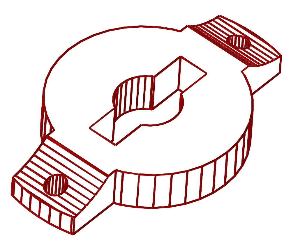
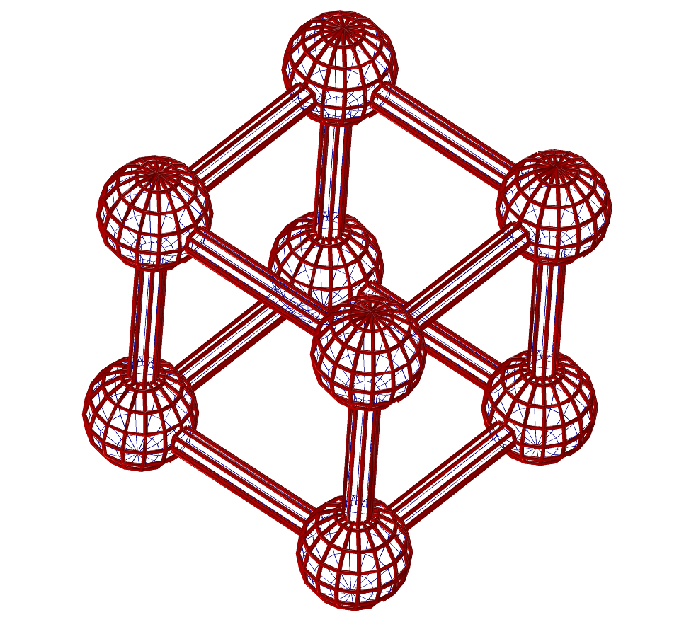
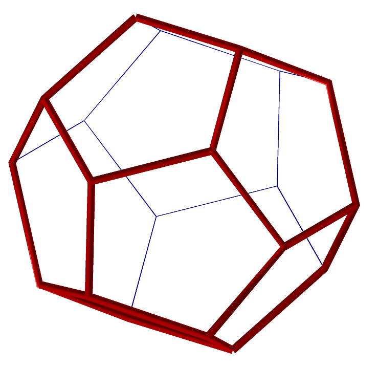
FIGURE:
Some examples of the use of the hidden line removal tool, poly3d-h,
to remove hidden lines.
The program performs 4 passes over the input:
1. Preprocesses and maps all polygons in a scene, and sorts them.
2. Generates edges out of the polygonal model and sorts them (preprocessing
for the scan line algorithm) into buckets.
3. Intersects edges, and splits edges with non-homogeneous visibility (the
scan line algorithm).
4. Applies a visibility test on each edge.
This program can handle CONVEX polygons only. From IRIT one can
ensure that a model consists of convex polygons only, using the CONVEX
command:
CnvxObj = convex( Obj );
just before saving it into a file. Surfaces are always decomposed into
triangles.
poly3d-h output is in the form of polylines. It is a regular IRIT
data file that can be viewed using any of the display devices, for example.
Command Line Options
poly3d-h [-b] [-m] [-i] [-e #Edges] [-H] [-4] [-W Width]
[-F PolyOpti FineNess] [-q] [-o OutName] [-t AnimTime]
[-c] [-z] DFiles > OutFile
-b: BackFacing - if an object is closed (such as most models created by
IRIT), backfacing polygons can be deleted, thereby speeding up
the process by at least a factor of two.
-m: More - provides some more information on the parsed data file(s).
-i: Internal edges (created by IRIT) - default is not to
display them, and this option will force their display, as well.
-e n: Number of edges to use from each given polygon (default all).
Handy as '-e 1 -4' for freeform data.
-H: Dumps both visible lines and hidden lines as separated objects.
Hidden lines will be dumped using a different (dimmer) color and (a
narrower) line width.
-4: Forces four polygons per almost flat region in the surface to
polygon conversion. Otherwise two polygons only.
-W Width: Selects a default width for visible lines in inches.
-F PolyOpti FineNess: Optimality of polygonal approximation of
surfaces. See the variable POLY_APPROX_OPT for the meaning of
FineNess. See also -4.
-q: Quiet mode. No printing aside from fatal errors. Disables -m.
-o OutName: Name of output file. Default is stdout.
-t AnimTime: If the data contains animation curves, evaluate and
process the scene at time AnimTime.
-z: Prints version number and current defaults.
-c: Clips data to screen (default). If disabled ('-c-'), data
outside the view screen ([-1, 1] in x and y) are also processed.
Some of the options may be turned on in poly3d-h.cfg. They can then be
turned off in the command line as '-?-'.
Configuration
The program can be configured using a configuration file named poly3d-h.cfg.
This is a plain ASCII file you can edit directly and set the parameters
according to the comments there. 'poly3d-h -z' will display the current
configuration as read from the configuration file.
The configuration file is searched in the directory specified by the
IRIT_PATH environment variable. For example,
'setenv IRIT_PATH /u/gershon/irit/bin/'.
If the IRIT_PATH variable is not set, the current directory is searched.
Usage
As this program is not interactive, usage is quite simple, and the only
control available is the command line options.
If a certain surface should be polygonized into a finer/coarser
set of polygons than the rest of the scene, one can set a "resolution"
attribute which specifies the relative FineNess resolution of this
specific surface. Further, "u_resolution" and "v_resolution" might be
similarly used to set relative resolution for the u or v direction only.
The "crv_resolution" attribute controls the relative fineness of curves
as polylines. The "num_of_isolines" attribute controls the relative number
of isoparametric curves.
See also IHidden.
Illustrt - Simple line illustration filter
Introduction
illustrt is a filter that processes IRIT data files and dumps out modified
IRIT data files. illustrt can be used to make simple, nice illustrations of
data. The features of illustrt include depth sorting, hidden line clipping
at intersection points, and vertex enhancements. illustrt is designed to
closely interact with irit2ps, although it is not neceessary to use irit2ps
on illustrt output.
See figure for an example.
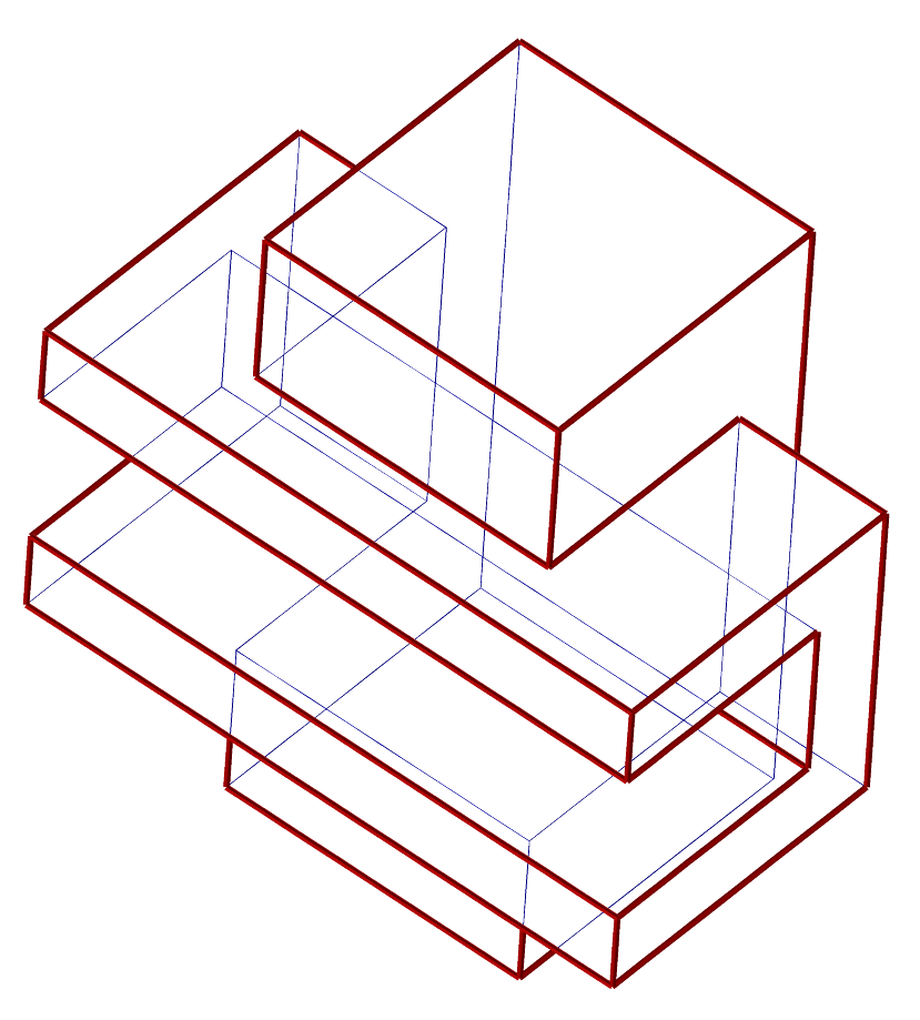
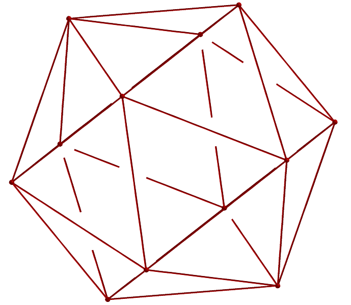
FIGURE:
Some examples of the use of the illustration tool, illustrt.
Command Line Options
illustrt [-I #UIso[:#VIso[:#WIso]]] [-f PolyOpti SampTol] [-s] [-M] [-P]
[-p] [-O] [-l MaxLnLen] [-a] [-t TrimInter] [-o OutName]
[-Z InterSameZ] [-m] [-T AnimTime] [-z] DFiles
-I #UIso[:#VIso[:#WIso]]: Specifies the number of isolines per
surface/trivariate, per direction. If #VIso is not specified,
#UIso is used for #VIso as well and so no.
-f PolyOpti SampTol: Controls the method used to approximate curves
into polylines. If PolyOpti == 0, equally spaced intervals are
used. For PolyOpti == 1, SampTol (real number) specifies the
maximal allowed deviation tolerance of the piecewise linear
approximation from the original curve.
Default is 0 64 (uniform sampling with 64 samples).
-s: sorts the data in Z depth order that emulates hidden line removal
once the data are drawn.
-M: Dumps the control mesh/polygon as well.
-P: Dumps the curve/surface as isocurves.
-p: Dumps vertices of polygons/lines as points.
-O: Handles polygonal objects as possibly open. This will generate
two identical edges for an edge shared by two adjacent polygons.
This can be useful for open or isolated polygons.
-l MaxLnLen: Breaks long lines into shorter ones with maximal length
of MaxLnLen. This option is necessary to achieve good depth depending
on line width in the '-d' option of irit2ps.
-a: Takes into account the angle between the two (poly)lines that
intersect when computing how much to trim. See also -t.
-t TrimInter: Each time two (poly)line segments intersect in the
projection plane, the (poly)line that is farther away from the
viewer is clipped by the TrimInter amount from both sides. See also -a.
-o OutName: Name of output file. Default is stdout.
-Z InterSameZ: The maximal Z depth difference of intersection curves
to be be considered invalid.
-m: More talkative mode. Prints processing information.
-T AnimTime: If the data contain animation curves, evaluate and
process the scene at time AnimTime.
-z: Prints version number and current defaults.
Usage
illustrt is a simple line illustration tool. It processes geometry such
as polylines and surfaces and dumps geometry with attributes that will make
nice line illustrations. illustrt is geared mainly toward its use with
irit2ps to create postscript illustrations. Here is a simple example:
illustrt -s -l 0.1 solid1.itd | irit2ps -W 0.05 -d 0.2 0.6 -u - > solid.ps
makes sure all segments piped into irit2ps are shorter than 0.1 and sorts them
in order to make sure hidden surface removal is correctly applied. Irit2ps
is invoked with depth cueing activated, and a default width of 0.05.
illustrt dumps out regular IRIT data files, so output can be handled
like any other data set. illustrt does the following processing to the input
data set:
Converts surfaces to isocurves ('-I' flag) and isocurves and curves to
polylines ('-S' flag), and converts polygons to polylines.
Polygonal objects are considered closed and even though each edge is
shared by two polygons, only a single one is generated.
Finds the intersection location in the projection plane of all segments in
the input data set and trims away the far segment at both sides of the
intersection point by an amount controlled by the '-t' and '-a' flags.
Breaks polylines and long lines into short segments, as specified via the
'-l' flag, so that width depth cueing can be applied more accurately
(see irit2ps's '-d' flag) as well as the Z sorting.
Generates vertices of polygons in the input data set as points in output data
controlled via the '-p' flag.
set.
Applies a Z sort to the output data, if '-s', so drawing in order of the data
will produce a properly hidden surface removal drawing.
Here is a more complex example. Make sure tubular is properly set via
"attrib(solid1, "tubular", 0.7);" and invoke:
illustrt -s -p -l 0.1 -t 0.05 solid1.itd |
irit2ps -W 0.05 -d 0.2 0.6 -p h 0.05 -u - > solid.ps
makes sure all segments piped into irit2ps are shorter than 0.1, generates
points for the vertices, sorts the data in order to make sure hidden surface
removal is correctly applied, and trims the far edge by 0.05 at an
intersection point. Irit2ps is invoked with depth cueing activated and a
default width of 0.05, points are drawn as hollowed circles of default
size 0.05, and lines are drawn tubular.
Objects in the input stream that have an integer attribute by the
name of "IllustrtNoProcess" are passed to the output unmodified. If
this attribute value is <= 0, the object is sent to the output stream
immediately (in the beginning of the output stream. If this
attribute value is > 0, the object is sent to the output stream at
the end (in the end of the output stream.
Objects in the input stream that have a real attribute by the name of
"IllustrtShadeBG" are copied and rendered also in the background
with a gray color as set by this attribute (between zero and one). If
a regular color/rgb attribute is found on the object, this value will
scale that as well.
Objects in the input stream that have an attribute by the name of
"SpeedWave" will have a linear segment added that emulates fast
motion with the following attributes,
"Randomness,DirX,DirY,DirZ,Len,Dist,LenRandom,DistRandom, width".
Objects in the input stream that have an attribute by the name of
"HeatWave" will have a spiral curves added that emulate a heat wave
in the +Z axis with the following attributes,
"Randomness,Len,Dist,LenRandom,DistRandom, width".
Examples:
attrib(Axis, "IllustrtNoProcess", 1);
attrib(Srf, "IllustrtShadeBG", 0.7);
attrib(Obj, "SpeedWave", "0.0005,1,0,0,5,3,3,2,0.05");
attrib(Obj, "HeatWave", "0.015,0.1,0.03,0.06,0.03,0.002");
Aisoshad - Simple line illustration filter
Introduction
Aisoshad is a filter that processes IRIT data files of freeform shapes
and dumps out modified IRIT data files in the form of short
univariate strokes. Aisoshad can be used to make simple yet nice line
art illustrations of geometry that is based solely on isoparametric
curves.
Aisoshad employs a simple shader to determine the density of the
isoparametric strokes as well as the thickness etc. Output of aisoshad
can be piped into the irit2ps postscript postprocessor.
See figure for an example.
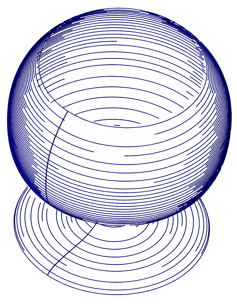
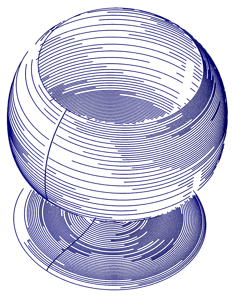
FIGURE:
Examples of the use of the aisoshad illustration tool to
line art illustrative drawing using isoparametric curves. In (left),
silhouettes are emphasized, while in (right) a light source above and to
the right is placed using a cosine shader.
Command Line Options
aisoshad [-o OutName] [-m] [-i] [-F PolyOpti FineNess]
[-f PolyOpti SampTol] [-r RndrMdl] [-c CosPwr] [-s SdrPwr]
[-l Lx Ly Lz] [-R Random] [-d AdapDir] [-t SrfZTrans]
[-M MinSubdiv] [-D AdapDist] [-w AdapIsoWidth] [-S WidthScale]
[-W] [-u] [-Z ZbufSize] [-b] [-z] DFiles
-o OutName: Name of output file. Default is stdout.
-m: More talkative mode. Prints processing information.
-i: Solve symbolic products using interpolations. Faster but the
generated output is not as compact as possible.
-I #IsoLines: Specifies number of isolines per surface, per direction.
-F PolyOpti FineNess: Optimality of polygonal approximation of
surfaces. See the variable POLY_APPROX_OPT for the meaning of
FineNess. Default is 0 and 20.0 (no optimal sampling with fineness
of 20.0 (real number)).
-f PolyOpti SampTol: Controls the method used to approximate curves
into polylines. If PolyOpti == 0, equally spaced intervals are
used. For PolyOpti == 1, SampTol (real number) specifies the
maximal allowed deviation tolerance of the piecewise linear
approximation from the original curve.
Default is 0 64 (uniform sampling with 64 samples).
-r: Selects the rendering model of the shader as follows:
1. Cosine shader, diffuse only, light source regular.
2. Cosine shader, diffuse only, light source as two lights from
opposite directions.
3. Cosine shader, has specular term, light source regular.
4. Cosine shader, has specular term, light source as two lights.
5. Shader emphasizing the silhouette areas of the model.
6. Shader estimating distance decay from a point light source.
-c CosPower: Controls the cosine shader's power.
-s SdrPower: Controls the shader's relative influence.
-l Lx Ly Lz: Sets the light source position/direction.
-R Random: Controls the levels of randomness that the isoparametric
curves perturb. Low levels of randomness would leave visible
artifacts while too high levels would disturb the shading. Should be
greater than one or negative one to disable.
-d AdapDir: Sets the isoparametric directions of the strokes. Either
0, 1, or 2 for U direction, V direction or both U and V directions,
respectively.
-t SrfZTrans: The amount to translate the created line strokes in Z,
in order to prevent Z fighting with the rendered object itself.
-M MinSubdiv: Sets the minimal number of subdivision to enforce
during the isoparametric strokes' construction. This flag should be
used rarely and typically MinSubdiv should be low and close to one.
-D AdapDist: Sets the distance between adjacent isocurves. The smaller
AdapDist is, the denser the coverage of the strokes will be.
-w AdapIsoWidth: Sets the default width attribute of the generated
strokes.
-S WidthScale: Controls the relative variance of the width of the
strokes in variable width strokes.
-W: If set, enables variable width strokes.
-u: If set, maps the strokes to screen space. Otherwise, strokes
are mapped back to object space.
-Z ZbufSize: Sets the size of the (square) Z buffer to set.
-b: If set, generates a binary IRIT data file that holds the
strokes. Otherwise, IRIT text file will be created.
-z: Print version number and current defaults.
Usage
Aisoshad is a simple line art illustration tool that generates strokes
that follow the isoparametric curves. It processes freeform geometry such
as surfaces and dumps geometry with attributes that makes
nice line illustrations. Aisoshad is geared mainly toward its use with
irit2ps to create postscript illustrations. Here is a simple example:
aisoshad -Z -500 -F 0 50 -s 10 -c 1 -D 0.3 -r 5 wglass.itd view.imd |
irit2ps -W 0.05 -d 0.2 0.6 -u - > wglass1.ps
that creates line art illustrations of a wine glass wglass.itd with
hidden strokes removed via a Z-buffer of size 500 that will be displayed on
screen, polygonal fineness of 50 for the surface of the glass, shader power
of 10 and cosine power of 1, isoparametric curves maximal distance of 0.3,
and shader number 5 that emphasizes silhouettes. The output of the shader
is piped to a irit2ps filter to postscript that sets the width of the strokes
to be a function of depth.
Here is another example:
aisoshad -Z 700 -R 4 -F 0 50 -l 1 1 1 -D 0.02 -r 2 wglass.itd view.imd
irit2ps -W 0.005 -d 0.2 0.6 -u - > wglass2.ps
that creates line art illustrations of a wine glass wglass.itd with
hidden strokes removal via a Z-buffer of size 700 that is allocated off-line
in core memory, polygonal fineness of 50 for the surface of the glass,
a light source at (1, 1, 1), isoparametric curves maximal distance of 0.02,
and a cosine shader number 2. The output of the shader is piped to a irit2ps
filter to postscript that sets the width of the strokes to be a function of
depth.
Transparent objects, or objects with the "transp" attribute, would generate
strokes as regular surfaces but would not participate in the hidden strokes
removal. An "AdapIsoDir" attribute that is found on some surface object
would override the global isoparametric direction's setup of strokes as is
set via the 'd' option.
See also the illustrt, izebra, lineshad, and
irit2ps tools.
IZebra - Simple zebra style, parallel curve based rendering
Introduction
Izebra is a filter that processes IRIT data files into a 2D striped,
zebra style illustration that gives the user an illusionary depth cue. The
output is also an IRIT data file in the form of freeform curves. Izebra
can be used to make simple yet nice art illustrations of geometry that is
based on a specific style inspired by the artist Victor Vasarely.
Izebra employs a Z buffer to determine the density and warping of the
stripes. Output of izebra can be piped into the irit2ps postscript
postprocessor.
See figure for an example.
FIGURE:
Examples of the use of the izebra illustration tool toward
line art illustrative drawings. On the left, the Utah teapot is
rendered, while on the right, a chess piece, a pawn, is portrayed.
Command Line Options
IZebra [-o OutName] [-m] [-O ImgOper] [-F PolyOpti FineNess] [-u]
[-I NumIters] [-Z ZbufSize] [-B CbcBspSize] [-D DataSrf]
[-A StripeAngle] [-b] [-s Stripes] [-S ZScale] [-d ZInitDepth]
[-z] DFiles
-o OutName: Name of output file. Default is stdout.
-m: More talkative mode. Prints processing information.
-O ImgOper: By default, the Z buffer is employed directly. However,
once the Z buffer is fully evaluated and before beginning the stripes
processing, one can apply a filter to the Z map of the Z buffer. The
filter can be a first order Roberts derivative if "-O 1", a second
order Laplacian if "-O 2", or an inverted depth if "-O 3".
-F PolyOpti FineNess: Optimality of polygonal approximation of
surfaces. See the variable POLY_APPROX_OPT for the meaning of
FineNess. Default is 0 and 20.0 (no optimal sampling with fineness
of 20.0 (real number)).
-u: Forces a unit matrix. That is, input data are not
transformed at all.
-I NumIters: Puts a bound on the number of iterations in the
numerical processing stage.
-Z ZbufSize: ZbufSize sets the size of the (square) Z buffer to set.
-B CbcBspSize: Sets the mesh size of the constructed uniform cubic
B-spline grid, if no data surface is specified by '-D'.
-D DataSrf: If specified, provides the name of the uniform cubic
B-spline to load and warp. Overrides the '-B' option.
-A StripeAngle: Sets the angle of the stripes with respect to the
horizontal line, in degrees.
-b: If set, generates a binary IRIT data file that holds the
stripes. Otherwise, an IRIT text file will be created.
-s Stripes: If set, prescribes the number of strips to extract as iso
parametric curves of the warped B-spline surface. Otherwise, the
warped B-spline surface itself is dumped out.
-S ZScale: A relative factor to control the effect of the depth
on the warping amount. This should be around one.
-d ZInitDepth: By default, the Z buffer is initialized to a depth of
zero which amounts to no warping of the B-spline surface. Here is
a proper way to prescribe a different background depth (which will
cause warping in the surface).
-z: Print version number and current defaults.
Usage
Izebra is a simple stripes art illustration tool that generates stripes
that follow a warped B-spline surface as its isoparametric curves. It
processes the given geometry, such as surfaces, into a Z map of a Z buffer
and warps a B-spline surface that is placed over it, with a warping amount
that is a function of the locally detected depth. IZebra dumps out stripes
geometry that makes nice illusionary illustrations. IZebra is geared
mainly toward its use with irit2ps to create postscript illustrations.
Here is a simple example:
izebra -m -Z 500 -B 150 -I 10 -F 0 100 -A 140 -S 0.35 pawn.itd |
irit2ps -f 0 300 -u -B -0.45 -0.75 0.65 0.75 -W 0.004 -I 0:250 - > pawn.ps
creates striped illustrations of a pawn chess piece, with the aid
of a Z-buffer of size 500 by 500, a uniform cubic B-spline surface with mesh
size of 150 by 150, polygonal fineness of 100 for the surface of the pawn,
rotation of stripes of 140 degrees and Z scale factor of 0.35. Ten iterations
will be conducted during the numerical processing of the data.
The output of izebra is piped by the irit2ps filter to postscript that
extracts 250 isoparametric curves out of the dumped warped surface and sets
the width of the strokes to be 0.004.
Here is another example:
izebra -m -Z 500 -B 200 -I 10 -F 0 100 -A -90 -S 0.4 teapot.itd |
irit2ps -f 0 200 -u -B -0.55 -0.35 0.55 0.35 -W 0.007 -I 0:150 - > teapot.ps
creates striped illustrations of the Utah Teapot, with the aid
of a Z-buffer of size 500 by 500, a uniform cubic B-spline surface with mesh
size of 200 by 200, polygonal fineness of 100 for the surface of the teapot,
rotation of stripes of -90 degrees and Z scale factor of 0.4. Ten iterations
will be conducted during the numerical processing of the data.
The output of izebra is piped by the irit2ps filter to postscript that
extracts 150 isoparametric curves out of the dumped warped surface and sets
the width of the strokes to be 0.007.
See also the illustrt, aisoshad, lineshad, and
irit2ps tools.
LineShad - Simple line illustration filter
Introduction
Lineshad is a filter that processes IRIT data files of freeform shapes
and dumps out modified IRIT data files in the form of short
univariate strokes. Lineshad can be used to make simple yet nice line
art illustrations of geometry that is based on arbitrarily stroked
curves on the surfaces.
Lineshad employs a simple shader to determine the density of the
isoparametric strokes as well as the thickness etc. Output of lineshad
can be piped into the irit2ps postscript postprocessor.
See figure for an example.
FIGURE:
Examples of the use of the lineshad illustration tool to
line art illustrative drawing using isoparametric curves. On the left,
silhouettes are emphasized, while on the right, a light source above
and to the right is placed using a cosine shader.
Command Line Options
lineshad [-o OutName] [-m] [-F PolyOpti FineNess] [-R RelStepSize]
[-f PolyOpti SampTol] [-r RndrMdl] [-c CosPwr] [-s SdrPwr]
[-i Intensity] [-l Lx Ly Lz] [-v Vx Vy Vz] [-w Width]
[-d Density] [-t SrfZTrans] [-S WidthScale] [-T Texture]
[-Z ZbufSize] [-b] [-z] DFiles
-o OutName: Name of output file. Default is stdout.
-m: More talkative mode. Prints processing information.
-F PolyOpti FineNess: Optimality of polygonal approximation of
surfaces. See the variable POLY_APPROX_OPT for the meaning of
FineNess. Default is 0 and 20.0 (no optimal sampling with fineness
of 20.0 (real number)).
-R RelStepSize: Relative control (default to 1.0) on the step size
taken during the numerical marching on the surfaces in the different
strokes' patterns.
-f PolyOpti SampTol: Controls the method used to approximate curves
into polylines. If PolyOpti == 0, equally spaced intervals are
used. For PolyOpti == 1, SampTol (real number) specifies the
maximal allowed deviation tolerance of the piecewise linear
approximation from the original curve.
Default is 0 64 (uniform sampling with 64 samples).
-r: Selects the rendering model of the shader as follows:
1. Dumps only the uniform point distribution.
2. Cosine shader, diffuse only, light source regular.
3. Cosine shader, diffuse only, light source as two lights from
opposite directions.
4. Cosine shader, has specular term, light source regular.
5. Cosine shader, has specular term, light source as two lights.
6. Shader emphasizing the silhouette areas of the model.
7. Shader estimating distance decay from a point light source.
-c CosPower: Controls the cosine shader's power.
-s SdrPower: Controls the shader's relative influence.
-i Intensity: Controls the global density of the constructed line art.
The larger Intensity is, the denser the drawing becomes.
-l Lx Ly Lz: Sets the light source position/direction.
-v Vx Vy Vz: Sets the viewing direction; typically, the Z axis.
-w Width: Sets the width of the generated strokes.
-d Density: Relative control (default to 1.0) of the density of the
uniform point distribution from which the strokes are developed.
-t SrfZTrans: Amount of created line strokes in Z to translate,
in order to prevent Z from fighting with the rendered object itself.
-S WidthScale: Controls the relative variance of the width of the
strokes in variable width strokes.
-T Textures: Selects the pattern of the strokes. Texture can be one
of:
1. "isoparam[,{0,1,2}w]": Isoparametric curves will be created in
a similar way to the aisoshad tool. Following the "isoparam"
string, one can optionally specify the isoparametric direction
as 0, 1 or 2 for U, V, or both, and a second 'w' character for
optional variable width. This option extracts exact
isoparametric curves from the given surface.
2. "wood[,Dx,Dy,Dz]": A strokes' style following layers of wood
will be used. Optionally, a direction normal to the layers
can be specified, with a default being the Z axis.
3. "vood[,Ry,Rz]": A variation on the wood texture, this time with
a layered orientation set via two rotation angles around Y and
Z.
4. "isomarch[,{0,1,2}]": Similar to "isparam" but numerically
march on the surface in the isoparametric direction. Again,
0, 1, or 2 stands for U, V, or both isoparametric directions.
5. "silhouette[,{t,n,tn}]": Extract strokes emphasizing the
silhoeutte areas from the given viewing direction. Strokes
can be extracted in the direction of the surface normal near
the silhouette area if option ",n" is given, tangent along
the surface if ",t", or both if ",tn".
6. "iTexture": Employ a raster image as a texture image on the
surface with the gradient of the image serving as the strokes
direction. The name of the image itself (must be in urt rle
format) is expected in a "iTexture" attribute on the specific
object.
7. "curvature[,{0,1,2}]": Develop strokes along lines of
curvatures. Strokes are developed along the minimal curvature
if ",0", the maximal curvature if ",1", and both if ",2".
8. "CurveStroke": An XY curve object is expected as a
"CurveStroke" attribute on the same object and serves as a
specification of motion in the parametric space of the surface
for each given point.
-Z ZbufSize: ZbufSize sets the size of the (square) Z buffer to set.
-b: If set, generates a binary IRIT data file that holds the
strokes. Otherwise, an IRIT text file will be created.
-z: Print version number and current defaults.
Usage
lineshad is a simple line art illustration tool that generates strokes
that follow the isoparametric curves. It processes freeform geometry such
as surfaces, and dumps geometry with attributes that makes
nice line illustrations. lineshad is geared mainly toward its use with
irit2ps to create postscript illustrations. Here is a simple example:
lineshad -Z -500 -F 0 50 -T "isoparam" -d 0.5 -c 10 -r 2 wglass.itd view.imd |
irit2ps -W 0.002 -u - > wglass3.ps
creates line art illustrations of a wine glass wglass.itd with
hidden strokes removal via a Z-buffer of size 500 that will be displayed on
screen, polygonal fineness of 50 for the surface of the glass, shader that
employs isoparametric curves, relative density of distribution of 0.5, and
cosine power of 10 of the cosine shader number 2.
Here is another example:
lineshad -Z -500 -F 0 50 -T "wood,1,1,1" -d 6 -c 10 -r 2 wglass.itd view.imd |
irit2ps -W 0.002 -u - > wglass4.ps
creates line art illustrations of a wine glass wglass.itd with
hidden strokes removal via a Z-buffer of size 500 that is allocated off-line
in core memory, polygonal fineness of 50 for the surface of the glass,
a light source at (1, 1, 1) for the wood strokes' style, relative point
distribution of 6, and a cosine power of 10 for the cosine shader number 2.
Transparent objects, or objects with the "transp" attribute, will generate
strokes as regular surfaces but will not participate in the hidden strokes
removal. A string "itexture" attribute is expected if "itexture" strokes'
style is used. A curve object as the "CurveStroke" attribute is expected if
"CurveStroke" is employed. One can override the strokes' style as it is set
via the '-T' command line option by setting an "lTexture" string attribute
with the prefered strokes' style of this object. One can modify the relative
density of some specific object by placing a real number attribute named
"PtsDensity" on the object.
See also the illustrt, izebra, aisoshad, and
irit2ps tools.
ihidden - Hidden Curve Removing Program
Introduction
ihidden is a program to remove hidden curves from a given surface model.
Only freeform objects are processed in ihidden.
See figure for an example.
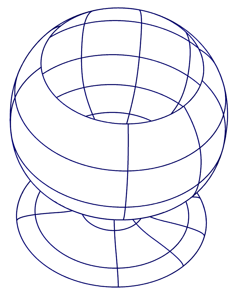
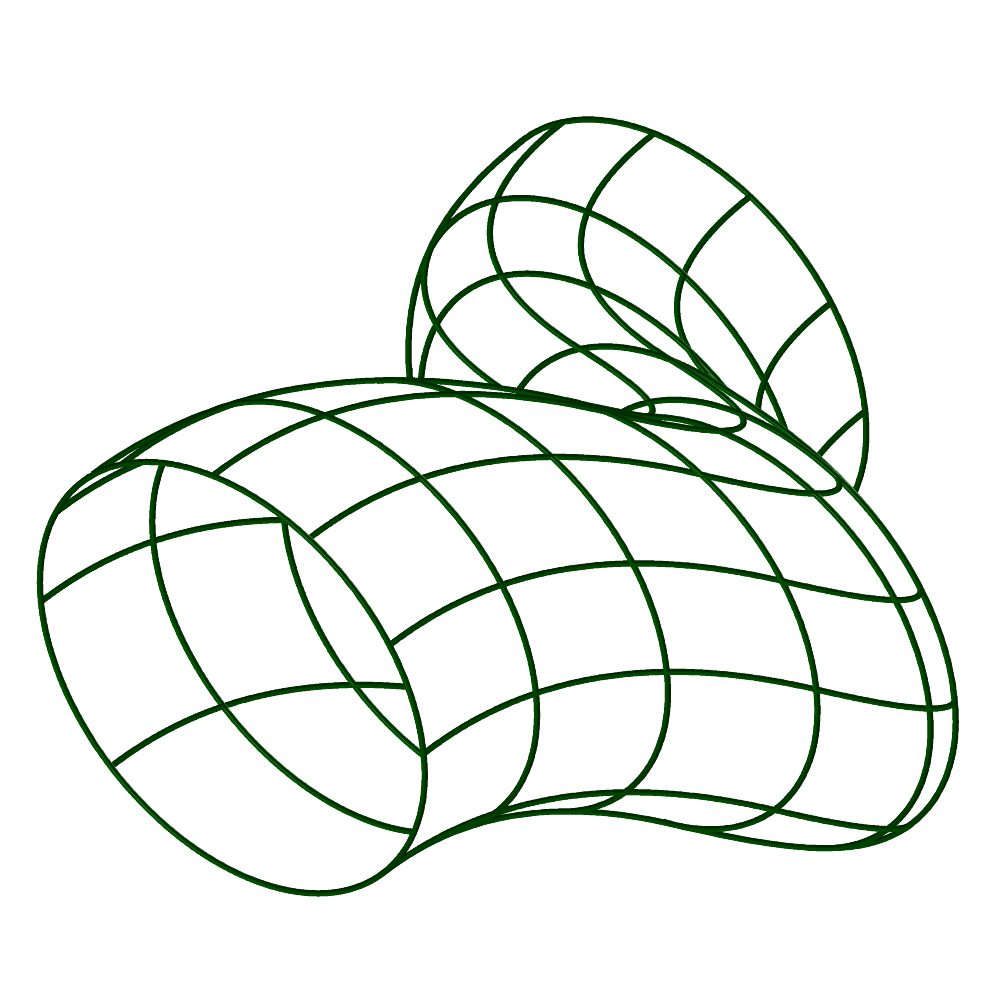
FIGURE:
Some examples of the use of hidden curve removal tool, ihidden, to
remove hidden curves.
The program performs 3 passes over the input:
1. Preprocesses and extracts the different curves in a scene, boundary curves,
silhouette curves, isoparametric curves and discontinuity curves.
2. Solves for all the intersections of the different curves in the parametric
space, and at that point splits the curves into curve segments.
3. Applies a visibility test to each segment of curve.
This program can handle non self interesecting surfaces only. Further,
surfaces that intersect other surfaces and are not properly trimmed into
a model are likely to result in the wrong answer as well.
The output of ihidden is in the form of curves. It is a regular
IRIT data file that can be viewed using any of the display
devices, for example.
Command Line Options
ihidden [-q] [-H] [-M] [-I #UIso[:#VIso[:#WIso]]] [-d] [-s Stage] [-b]
[-o OutName] [-t Tolerance] [-Z ZBufSz] [-T AnimTime] [-z] DFiles
-q: Quiet - provides no information on the progress if TRUE.
-H: Dumps both visible lines and hidden curves as separated objects.
Hidden curves will be dumped using a narrower line width.
-M: Force conversion of (active) curves to be monotone.
-I #UIso[:#VIso[:#WIso]]: Specifies the number of isolines per
surface/trivariate, per direction. If #VIso is not specified,
#UIso is used for #VIso as well and so on.
-d: Add to also display C1 discontinuity curves.
-s: Specifies the step at which to stop this process, where step 3, as
described above, will complete the entire hidden curve removal
process and is the default.
-b: If set, generates a binary IRIT data file that holds the
strokes. Otherwise, an IRIT text file will be created.
-o OutName: Name of output file. Default is stdout.
-t Tolerance: Tolerance of computation.
-Z ZBufSz: Size of the Z buffer in the visibility testing process.
-T AnimTime: If the data contains animation curves, evaluate and
process the scene at time AnimTime.
-z: Prints version number and current defaults.
Some of the options may be turned on in ihidden.cfg. They can then be
turned off in the command line as '-?-'.
Configuration
The program can be configured using a configuration file named ihidden.cfg.
This is a plain ASCII file you can edit directly and set the parameters
according to the comments there. 'ihidden -z' will display the current
configuration as read from the configuration file.
The configuration file is searched in the directory specified by the
IRIT_PATH environment variable. For example,
'setenv IRIT_PATH /u/gershon/irit/bin/'.
If the IRIT_PATH variable is not set, the current directory is searched.
Usage
As this program is not interactive, usage is quite simple, and the only
control available is using the command line options.
If a certain surface should contain more or less isoparametric curves,
a relative change could be applied to some specific object via the
"num_of_isolines" attribute. If a "transp" attribute is found on some
object, it will generate all the curves but will not affect the visibility
(i.e. be fully transparent).
See also Poly3d-h.
Irender - Simple Scan Line Renderer
Introduction
irender is a program to render IRIT scenes into images. It is
a software based Z buffer that is able to create images in few formats.
Several of its features includes parametric and volumetric texture mapping,
shadow computations, transparency and antialiasing.
Freeform objects are preprocessed into polygons with controlled fineness.
See figure for an example.
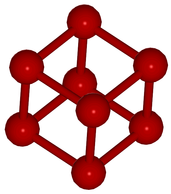
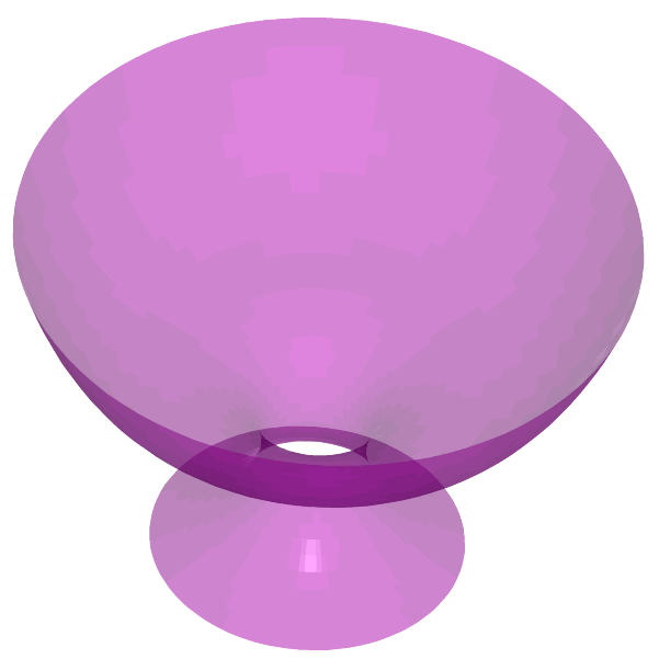
FIGURE:
Some examples of the use of irender scan convertion tool to render
images of IRIT scenes. Highlights can be seen in the
molecule image while the glass is rendered transparent.
Command Line Options
irender [-v] [-s XSize YSize] [-Z Znear Zfar] [-a Ambient] [-b R G B]
[-B] [-F PolyOpti FineNess] [-f PolyOpti SampPerCrv]
[-M Flat/Gouraud/Phong/None] [-p PtRad] [-P WMin [WMax]] [-S]
[-T] [-t AnimTime] [-N ClrQuant SilWidth [SilR SilG SilB]]
[-A FilterName] [-d] [-D] [-l] [-V] [-n] [-i rle/ppm{3,6}/png]
[-o OutName] [-z] files
-v: Verbose mode. Prints informative messages as it progresses.
-s XSize YSize: Sets the size of the output image, in pixels.
Default to 512x512.
-Z Znear Zfar: Sets the near and far cliping planes with default
of no clipping.
-a Ambient: Sets the ambient lighting fraction. Between zero (no
ambient lighting) and one. Default to 0.2.
-b R G B: Sets the background color. Each of thre R,G,B colors is
an integer value between zero and 255. Default to black.
-B: Apply back face culling. Somewhat faster, but only correct for
closed objects. Default is no back face culling.
-F PolyOpti FineNess: Optimality of polygonal approximation of
surfaces. See the variable POLY_APPROX_OPT for the meaning of
FineNess. Default is 0 and 20.0 (no optimal sampling with fineness
of 20.0 (real number)).
-f PolyOpti SampTol: Controls the method used to approximate curves
into polylines. If PolyOpti == 0, equally spaced intervals are
used. For PolyOpti == 1, SampTol (real number) specifies the
maximal allowed deviation tolerance of the piecewise linear
approximation from the original curve.
Default is 0 64 (uniform sampling with 64 samples).
-M Flat/Gouraud/Phong/None: Selects the shader to be used. Default to
Phong if has normals of vertices, Flat if no normals are found.
The None options exactly paints the objects with the given color,
applying no shader.
-p PtRad]: Width of rendered points (as spheres).
-P WMin [WMax]: Width of rendered polyline, in world units. If only
WMin is specified, all polylines are set to have WMin width. Otherwise,
if WMax is prescribed as well, polylines' width is set to be
proportional to their depth with WMax is the width of closest polyline
and WMin the farest polyline. Polylines and curves will be
ignored without the setting of this option.
-S: Enable shadow computation. No shadows will be rendered without -S.
The is no shadow support for this release of irender.
-T: Enable transparency computation. No transparent object will be
processed without -T.
-t AnimTime: If the data contains animation curves, evaluate and
process the scene at time AnimTime.
-N ClrQuant SilWidth [SilR SilG SilB]: Requests cartooN style
NPR rendering. Two effects could be activated using this option:
the colors could be quantized into ClrQuant levels or,
alternatively a value of zero for ClrQuant denotes no
quantization. Also, open boundaries and silhouettes could be
rendered if SilWidth > 0.0 at SilWidth polyline
width and optional color SilR SilG SilB.
-A FilterName: Selects an antialiasing filter. FilterName can be one
of 'none', 'box', 'triangle', 'quadratic', 'cubic', 'catrom',
'mitchell', 'gaussian', 'sinc, and 'bessel'. Default is 'none'.
-d: Output will be in the form of Z depth instead of a color image.
Output will be 32 bits depth instead of RGBA.
-V: Output will be in form of visibility map: a map in model's UV
coordinates that represents the visibility of the model from the
specified rendering direction.
-n: Reverses the normals of vertices and planes, globally.
-i rle/ppm{3,6}/png/itd: Selects output image type.
Currently the Utah Raster Toolkit's (URT) rle format is being
supported as well as the PPM and PNG formats.
PPM can be either P6 or P3 style.
If (geometry) ITD is selected, output type must be Z depth (-d) and
a grid of the geometry of the Z depth map is dumped as itd file.
-o OutName: Name of output file. By default the output goes to
stdout.
-z: Prints version number and current defaults.
Some of the options may be turned on in irender.cfg. They can be then
turned off in the command line as '-?-'.
Configuration
The program can be configured using a configuration file named irender.cfg.
This is a plain ASCII file you can edit directly and set the parameters
according to the comments there. 'irender -z' will display the current
configuration as read from the configuration file.
The configuration file is searched in the directory specified by the
IRIT_PATH environment variable. For example,
'setenv IRIT_PATH /u/gershon/irit/bin/'.
If the IRIT_PATH variable is not set, the current directory is searched.
Usage
As this program is not interactive, usage is quite simple, and the only
control available is using the command line options.
Advanced Usage
One can specify several attributes that affect the way the scene is
rendered. The attributes can be generated within IRIT.
See also the ATTRIB IRIT command.
Surface color is controlled on two levels. If the object has an RGB
attribute, it is used. Otherwise, a color as set via the IRIT
COLOR command. If a vertex of a poly object has an RGB attribute it
will overwrite the object's RGB color for that vertex.
If a certain surface should be finer/coarser than the rest of the
scene, one can set a "resolution" attribute which specifies the
relative FineNess resolution of this specific surface. Further,
"u_resolution" and "v_resolution" might be similarly used to set
relative resolution for the u or v direction only.
The "crv_resolution" attribute controls the relative fineness of curves
as polylines. The "num_of_isolines" attribute controls the relative number
of isoparametric curves.
Points are rendered as small spheres with size (radius) that is controlled
by the "width" attribute found on the object or the radius that is specified
by the '-p' option as default size.
Objects are rendered with no shading if "NoShading" attribute is found on
them.
Example:
attrib( Ball, "rgb", "255,0,0" );
color( Sphere, white );
The cosine exponent of the phong shader can be set for a specific
object via the SRF_COSINE attribute, with 128 as default value.
An object can affect its diffuse and specular components via the
DIFFUSE and SPECULAR real attributes, with 0.4 as default value.
Example:
attrib( Ball, "srf_cosine", 16 );
attrib( Ball, "diffuse", 0.7 );
attrib( Ball, "specular", 1.0 );
An object can be drawn transparent instead of opaque, if it has a
"transp" attribute. A transparent value of one denotes a completely
transparent object, while a value of zero means a completely opaque
object. Transparent objects will be rendered as such if and only if the '-T'
command line option is set.
Example:
attrib( final, "transp", 0.5 );
An object can have its silhouettes (and boundary curves) rendered if a
real "SilWidth" attribute with width larger than zero is specified.
"SilColor" will then set the color of the rendered outline curves. See
also '-N' which sets this option globally.
Several types of texture mapping are supported. Parametric texture may be
attached to a parametric surface where the prescribed image is mapped onto
the rectangular parametric domain of the surface.
The parametric texture may be applied with the following options:
'D' x y z Vector that will be rotated to Z along with the
texture coordinates. Applies to 'T' 1, 2 or 3.
Default to the Z axis.
'O' x y z a point to which that texture Origin will be translated.
Applies to 'T' 1, 2 or 3. Default to origin.
'S' Su Sv {Sw} Scales the coordinates in u and v. Scale
factors of 1.0 would cover the entire surface
once. Default to scale factors of 1.0. If Sw is
specified for a polygonal object, each polygonal is
locally scaled based on its maximal projection on
one of the main, XY XZ or YZ, planes.
If (Su = Sv = 0) for freeforms, the texture coords
are undergoing no scale at all (assuming image domain
of zero to one in all axes).
'A' a Angle of rotation in degrees of texture map with
respect to main axis. Applies to 'T' 1, 2 or 3.
Default to no rotations.
'T' TextureType with 0 denotes regular parametric texture,
1 denotes spherical coordinates,
2 denotes spherical bijective coordinates,
3 denotes cylinderical coordinates,
4 denotes planar coordinates.
Regular parametric texture employs the inherited surface parametrization
of the freeform surface and can only be used on parametric surfaces.
Spherical, cylinderical, and planar coordinate transformations are useable
for all types of geometry from polygons to freeform surfaces and is
fairly straightforward with the origin as set by 'O' being the center
of the mapping while the direction set by 'D' controls the north pole
of the sphere, the axis of the cylinder, and the normal of the plane.
Finally, the angle set by 'A' rotates the texture around this 'D' prescribed
axis.
The spherical bijective mapping is more complex. An object identical
to the textured object should be found as an "PTextureBijectObj" that
contains the identical topology of the original object. The original
object must be genus zero non convex, while the attribute object must be
a genus zero convex object with the origin as set via 'O', inside this
convex object. It is likely that both the original object and its attribute
object will be a polygonal object. Both objects must contain triangles only.
A bijective mapping is then conducted from every point on the original
non convex object to the convex attribute object and from there through
spherical mapping to the texture map.
Example:
attrib( Srf1, "ptexture", "checker.ppm, S 1 1, A 45" );
attrib( Srf2, "ptexture", "checker.ppm, S 1 3, T 1, O 1 1 1, D 0 0 1" );
attrib( Srf3Triangs, "ptexture", "checker.ppm, S 1 2, T 1, O 1 1 1, D 0 0 1" );
attrib( Srf3Triangs, "PTextureBijectObj", Srf3ConvexTriangles );
Srf1 is a parametrically textured map using spherical mapping,
Srf2 is a parametrically textured map using cylinderical
mapping and Srf3Triangs is a parametrically textured map using
spherical bijective mapping and Srf3ConvexTriangles is the convex
topologically equivalent object.
The program will automatically detect the image type according to
the file's type. Note that regular parametric texture may be applied to
parametric surfaces only, whereas the spherical, cylinderical and planar
parametric textures may be used on all types of geometry. Depending upon
the way irender is compiled, texture images could be in ppm format (always),
or gif, png, and rle. If the image has an alpha channel (fully supported
in png and rle and binary supported in gif images via its transparent color)
it is honored if transparency (-T) is activated.
A second type of texture mapping can be applied to all geometric objects.
Herein, a procedural texture mapping is employed. The currently supported
textures are
camouf Camouflage style
checker Checker style
chocolate Chocolate chips style
contour Parallel plane contouring
curvature Gaussian/Mean etc. curvature
marble Marble style
ncontour Constant normal angle to major axis
orange Bump mapping orange style
wood Wood style
punky Colorful punky style
A second parameter that must be provided for procedural textures is the
scaling factor of the texture, which can be either one parameter of uniform
scaling or a vector of three coefficients for scaling in x, y, and z.
For contour style, the scale denotes the spacing of the contouring
planes in X, Y and Z. For ncontour style, the scale also denotes
the spacing of the adjacent constant normal contours. Related attributes
are "texture_color" and "texture_width" that support the color and the
width of the textured strokes.
Example:
attrib( Obj1, "texture", "marble, 2" );
attrib( Obj2, "texture", "wood, 1 0.5 2.5" );
which sets Obj1 to have a marble procedural texture with a uniform
scaling factor of 2 and a wood texture for Obj2 with scaling factors
of (1, 0.5, 2.5) in x, y, and z.
In addition, the appearance of each procedural texture can be controlled by
optional parameters which are different for each texture. Each texture
parameter is recognized by a letter; to enter a parameter, add to the
attribute string the paramter letter followed by the value or values. Each
parameter should be separated by a comma.
Example:
attrib( Obj1, "texture", "wood, 2, b 0.3, o 5 5 5" );
sets Obj1 to have a wood procedural texture with a scaling factor
of 2, a Brightness level of 0.3, and the Origin point at (5,5,5).
The optional parameters are:
checker:
'z' x y z a vector to which the Z axis will be rotated.
'o' x y z a point to which the Origin will be translated.
'b' x the brightness of the checker color scaling,
should be between 0 and 1.
'CP' f To force a 2D checker plane orthogonal to the
vector that is specified via the 'z' option.
'C1' r g b A second optional color for the checkerboard.
'C2' r g b A third optional color for the checkerboard,
used in the second layer of the checker volume.
'C3' r g b A fourth optional color for the checkerboard,
used in the second layer of the checker volume.
chocolate:
'W' w the 'width' of chocolate piece (zero to half).
'd' x the 'depth' of the bumps on the bump-mapping.
contour:
'W' w the 'width' of contour.
'C' r g b the color of the contour in RGB betweeo zero
and one ("C 1 1 1" fully is white).
curvature:
The curvature texture has no optional parameter, but the first scale
parameter has a special meaning. A scale of
0 Paints convex regions in red, concave in
green, and saddle-like in yellow.
>0 Paints the Gaussian curvature in convex regions
in red to magenta, in concave regions in yellow
to green, and in saddle-like in cyan to blue.
<0 Paints the Mean curvature in positive mean
curvature regions in yellow to green and in
negative Mean curvature in red to magenta.
If this first scale parameter is non zero, its absolute value is used to
modify the blending speeds between the different colors.
marble:
'z' x y z a vector to which the Z axis will be rotated.
'o' x y z a point to which the Origin will be translated.
't' f s the scale of the turbulence noise, and the
factor to multiply that noise.
'f' x the 'frequency' of the marble layers.
ncontour:
'W' w the 'width' of contour.
'C' r g b the color of the contour in RGB betweeo zero
and one ("C 1 1 1" fully is white).
orange:
'd' x the 'depth' of the bumps on the bump-mapping.
wood:
'z' x y z a vector to which Z axis will be rotated.
'o' x y z a point to which the Origin will be translated.
'b' x the brightness of the wood color scaling,
should be between 0 and 1.
'c' f s the scale of the noise in the wood center axis
and the factor by which to multiply that noise.
'w' n f the number of angles to sample noise when creating
distortion in the circle shape of the wood
cylinders, and the factor by which to multiply that noise.
'f' x the 'frequency' of the wood cylinders.
'r' f s the scale of the wood-fibers noise, and the
factor by which to multiply that noise.
punky:
'b' x the brightness/saturation of the punky color.
More Examples:
attrib( Obj1, "texture", "marble, 2, t 3.0 12.0, f 7.0" );
attrib( Obj2, "texture", "contour, 1 0.5 2.5, W 0.004, C 1 1 0" );
sets Obj1 to have a marble procedural texture with a uniform
scaling factor of 2, and new turbulance and frequency factors.
This also sets a contouring texture for Obj2 with scaling
factors of (1, 0.5, 2.5) in x, y, and z, in yellow color and width 0.004.
In addition, a scalar surface spanning the same parameteric domain as an
original surface may be used as a texture mapping function. Herein, the
scalar function texture is evaluated at each UV parameter value and is mapped
through a color scale to yield the output color. This type of texture is
useful for stress maps or analysis maps on top of freeform surfaces.
Several related attributes are supported: "stexture_scale" which prescribes
the color scale image (only its first column is employed), and
"stexture_bound" that sets the domain that will be clipped to the min max
values. Funally, "stexture_func" can hold the functions "sqrt" or "abs"
to be applied to the evaluated surface value.
Example:
attrib( Srf, "stexture", scrvtr( Srf, P1, off ) );
attrib( Srf, "stexture_scale", "color_scale.ppm" );
attrib( Srf, "stexture_func", "sqrt" );
attrib( Srf, "stexture_bound", "0.0 100.0" );
where scrvtr computes a scalar field to Srf that represents the
sum of the squares of the principle curvatures. The evaluated scalar
texture surface's value is piped through a sqrt function.
The first column of the image of color_scale.ppm is used to set
the coloring scale for curvature bounds values between 0.0 and 100.0.
Both "stexture_scale" and "stexture_bound" are optional. The default
color scale maps the min/max values from blue to red through green. The
default scalar surface texture bound is computed as the extreme values of
the "stexture" surface.
While the program has a default for lighting which is two light
sources at opposite directions at (1, 1, 1) and (-1, -1, -1), one can
overwrite this default. A POINT_TYPE object with LIGHT_SOURCE
attribute denotes a light source. If irender detects one or more
light sources in the input stream, the default light sources are not
created. Two types of light sources may be prescribed, a parallel at
infinity or a point at a finite distance light source, distinguished
by a TYPE attribute of either POINT_POS or POINT_INFTY. A point
light source can be colored; an RGB attribute will set its (diffuse)
color. Specular color defaults to white but can be set via the
"SpecRGB" attribute. Ambient color defaults to black but can be set
via the "AmbtRGB" attribute. A point light source will cast shadows,
if and only if, it has a SHADOW attribute (one needs to apply the
'-S' command line option as well for rendering shadows). Finally, one
can construct two mirrored light sources at opposite directions if
the TWOLIGHT attribute is added to the light source object.
Example:
Light1 = point( 0, 0, 10 );
attrib( Light1, "light_source", on );
attrib( Light1, "shadow", on );
attrib( Light1, "rgb", "255,0,0" );
attrib( Light1, "type", "point_pos" );
Light2 = point( 1, 1, 1 );
attrib( Light2, "light_source", on );
attrib( Light2, "twolight", on );
attrib( Light2, "type", "point_infty" );
constructs two lights sources with Light1 with red color positioned
at (0, 0, 10) and casting shadows, while Light2 will create two
mirrored white parallel lights sources in the direction of (1, 1, 1) and
(-1, -1, -1), as its irender's default.
Visibility Maps
if the -V option is selected, the output will be a visibility map.
Visibility maps are created in the model's UV (texture) space and are
composed of 4 colors:
White: if pixel isn't mapped. I.e. the model UV's map does not cover this
pixel
Green: if the pixel is a (UV location of a Euclidean) visible location.
Red: if pixel is (UV location of a Euclidean) invisible location.
Yellow: if large errors are detected while calculating pixel's
visibility. This indeterministic result is due to almost
vertical polygns, typically.
Tips for geting higher quality visibility map:
1. Use the -s option for larger output resolution.
2. Use the -F option for finer polygonal sampling of surfaces.
Controlling the output can also be done by object attributes, as follow:
Use the 'tan_angle' property to change the yellow area of output. A
rendered triangle will be colored in yellow if it's surface is close
to being vertical, or tangent to the view, z, axis. Change the
'tan_angle' property to get maximal value of normalized scalar product
of triangle normal and z axis. Below that value the triangle will be
colored yellow. Default value: 0.1. Example:
attrib( Obj1, "tan_angle", 0.1 );
Use 'critic_ar' to change the unmapped area of output. Poor aspect ratio of
triangles leads to major errors. Aspect ratio is defined as the ratio of
largest edge by the smallest edge of triangle. Any triangle with aspect
ratio larger than 'critic_ar' will not be mapped.
Default value: 20.
attrib( Obj2, "critic_ar", 20 );
3DS2Irit - AutoCad 3DS Data To IRIT file filter
Converts '.3ds' data files to '.itd' IRIT data files.
Command Line Options
3ds2Irit [-m] [-c ClrScale] [-o OutName] [-b] [-z] 3DSFile
-m: More information flag.
-c ClrScale: Scaling the color values (intensity control).
-o OutName: Name of output file. By default the output goes to
stdout.
-b: If set, generates a binary IRIT data file that holds the
strokes. Otherwise, an IRIT text file will be created.
-z: Print version number and current defaults.
Usage
3ds2irit converts Autocad's 3DS data files into IRIT data files. The
current version provides only partial support, mainly due to lack of
documentation examples on the dxf format and the convoluted way
freeform surfaces are saved.
Example:
3ds2irit file.3ds > file.itd
Dat2Bin - Data To Binary Data file filter
Command Line Options
dat2bin [-t] [-z] {[-c QuantVal]} DFiles
-t: Dumps data to stdout as text instead of binary.
-z: Print version number and current defaults.
-c: Optional option that is available only if compressed binary files
are supported. Dumps data to stdout as compressed binary file
with a quanitization level of QuantVal.
Usage
The user may sometimes wish to convert .itd data files into a binary form,
for example, for fast loading of files with large geometry. Binary files can
be somewhat larger and are unreadable in editors but are much faster to load.
A binary file must have a '.ibd' file type.
Example:
dat2bin b58polys.itd > b58polys.ibd
dat2bin -t b58polys.ibd | more
The above converts a text file b58polys.itd into a binary file b58polys.ibd
and shows the content of the binary file by converting it back to text. At
this time data through pipes must be in text. That is, the following is
illegal:
dat2bin b58polys.itd | xglmdrvs -
It should be remembered that the binary format is not documented and
it might change in the future. Moreover, it is machine dependent and can
very well may be unreadable between different platforms.
Dat2Irit - Data To IRIT file filter
Converts '.itd' and '.ibd' data files to '.irt' IRIT scripts.
Optionally, if compressed binary files are supported, also handle
'.icd' compressed data files.
Command Line Options
dat2irit [-z] DFiles
-z: Print version number and current defaults.
Usage
Users may sometimes wish to convert .itd data files into a form that
can be fed back to IRIT - a '.irt' file. This filter does exactly that.
Example:
dat2irit b58.itd > b58-new.irt
Dxf2Irit - DXF (Autocad) To IRIT filter
Converts Autocad's, DXF data files into IRIT data files.
Command Line Options
dxf2irit [-m] [-f] [-o OutName] [-z] DXFFile
-m: Provides some more information on the data file(s) parsed.
-f: Coerces floating end conditions to constructed freeform surfaces.
Default is open end conditions.
-o OutName: Name of output file. By default the output goes to
stdout.
-z: Prints version number and current defaults.
Usage
dxf2irit converts Autocad's DXF data files into IRIT data files.
The current version provides only partial support for the conversion of
freeform surfaces, mainly due to lack of documentation examples on the
dxf format and the convoluted way freeform surfaces are saved.
Example:
dxf2irit file.dxf > file.itd
IGS2Irit - IGES Data To IRIT file filter
Converts '.igs' data files to '.itd' IRIT data files.
Command Line Options
IGS2Irit [-m] [-M] [-A] [-c] [-a] [-s] [-o OutName] [-b] [-z] IGSFile
-m: More information flag.
-M: Even more information flag - dumps all parsed entities.
-A: Allows the appproximated conversion of trimming curves with numerous
control points.
-c: Clips trimmed surfaces to the minimal domain as prescribed by the
trimming curves.
-a: Dumps all. Without this flag setting, only top level objects,
that are referenced by no other object, will be dumped out.
-s: Dumps surfaces only. When set only (trimmed) surfaces are dumped.
-o OutName: Name of output file. By default the output goes to
stdout.
-b: If set, generates a binary IRIT data file that holds the
data. Otherwise, an IRIT text file will be created.
-z: Print version number and current defaults.
Usage
igs2irit converts IGES data files into IRIT data files.
Example:
igs2irit file.igs > file.itd
Irit23js - Irit to ThreeJS filter
Command Line Options
irit23JS [-l] [-4] [-p] [-F PolyOpti FineNess] -i InName -o OutName
[-T] [-t AnimTime] [-z]
-l: Linear - forces linear (degree two) surfaces to be approximated
by a single polygon along their linear direction. Although
most of the time linear direction can be represented exactly
using a single polygon, even a bilinear surface can have a
freeform shape (saddle-like) that is not representable using
a single polygon. Note that although this option will better
emulate the surface shape, it will create unnecessary
polygons in cases where one is enough.
-4: Four - Generates four polygons per flat patch. Default is 2.
-p: for perspective camera, or orthographic camera otherwise.
-F PolygonOpti FineNess: Optimality of polygonal approximation
of surfaces. See the variable POLY_APPROX_OPT for the meaning
of FineNess. See also -4. Default FineNess is 20.
-o OutName: Specify the file path to the output file.
-i InName: Specify the file path to the input file.
-T: Talkative mode. Prints processing information.
-t AnimTime: If the data contains animation curves, evaluate and
process the scene at time AnimTime.
-z: Prints version number and current defaults.
Usage
Irit23js extracts the relevant data from Irit object files and
converts the object's polygon data to a format that can be loaded into
THREE.js via JSON file (see http://json.org/). The result is an HTML
file that can be used to view the Irit model in various web browsers
(Internet Explorer, Google Chrome, Firefox, Safari, etc), with help
from THREE.js, and using WebGL rendering.
Four files are created in all: three with a '.js' (JavaScript)
extension and one with an '.html' extension. Two of the JavaScript
files are required in order for the viewer to function properly. The
first is 'irit23js.js', which is a version of the THREE.js library,
and the second is 'iritOC.js', which is a THREE.js (Orbit Controls)
library that allows the user to pan, orbit, and zoom within the
viewer. These two files can be obtained by downloading the package
from the 'download' link on the three.js website (see
http://threejs.org/). The last JavaScript file is the actual geometry
output file that is written in JSON (JavaScript Object Notation)
format, and contains the polygon data for each object. Polygon data
exists in this JSON file as vertices, materials, textures, normals,
colors, UVs, and faces (refer to
https://github.com/mrdoob/three.js/wiki/JSON-Model-format-3 for an
explanation of this formatting). The HTML file allows the user to
directly view the model in the browser, as well as manipulate it with
the mouse and arrow keys if so desired.
In order to view the model in a web browser, the files must be
uploaded to a website, and all four of them should be placed in the
same web directory. This is the intended use, but if a user would
like to view the model from his/her file system, the HTML file must be
opened with Firefox or run locally through any web browser (IE,
Firefox, Chrome, Safari, etc). This restriction is a consequence of
the same-origin policy. A user attempting this second option should
take a look at the methods listed on this page:
https://github.com/mrdoob/three.js/wiki/How-to-run-things-locally.
If a model contained a texture in Irit, its image name within
irit23js has been modified to end with a '.jpg' extension, if it
wasn't already an image of that type. If the user wishes to see a
texture displayed on the model, the texture image must be placed in
the same directory as the above four output files, and its name must
match the one specified in the JavaScript file written in JSON (look
for the 'materials' property and the 'mapDiffuse' attribute).
Example:
irit23js -l -F 0 5 -i C:/irit/data/b58.itd -o C:/irit/b58.js
creates b58.js, b58Viewer.html, irit3js.js, and iritOC.js. The
model is created with low resolution (FineNess of 5). At such low
resolution, it may very well happen that triangles will have normals
"over the edge" since a single polygon may approximate a highly curved
surface. This problem will not arise if high fineness is used:
irit23js -l -F 0 30 -i C:/irit/data/b58.itd -o C:/irit/b58.js
creates ir_b58.js, ir_b58Viewer.html, irit3js.js, and iritOC.js. The
model is created with high resolution (FineNess of 30), so it will
have smooth curves and surfaces.
Advanced Usage
One can specify surface qualities for individual surfaces of a
model. Several such attributes are supported by irit23js and can be
set within IRIT. See also the ATTRIB IRIT command.
Example:
attrib( srf1, "resolution", 2 );
will force srf1 to have twice the default resolution, as set via the
'-F' flag.
Almost flat patches are converted to polygons. The rectangle can be
converted into two polygons (by subdividing along one of its
diagonals) or into four by introducing a new point at the patch
center. This behavior is controlled by the '-4' flag, but can be
overwritten for individual surfaces by setting "twoperflat" or
"fourperflat".
irit23js specific properties are controlled via the following
attributes: "transp" and "ptexture". The value of these attributes
must be strings as it is copied verbatim.
Example:
attrib( legs, "transp", "0.3" );
attrib( legs, "ptexture", "wood.jpg,2" );
attrib( table, "ptexture", "marble.jpg" );
An optional scale can be prescribed to textures. In the above example
wooden legs' (that are also transparent...) texture is selected with a
texture scaling factor of 2.
Surface color is controlled on two levels. If the object has an RGB
attribute, it is used. Otherwise a color as set via the IRIT COLOR
command is used, if set.
Example:
attrib( tankBody, "rgb", "244,164,96" );
Irit23mf - Irit to 3MF (3D Manufacturing Format) filter
Command Line Options
irit23mf [-l] [-4] [-F FineNess] [-w] [-i InName]
[-o OutName] [-z] [-d Designer]
-l: Linear - forces linear (degree two) surfaces to be approximated
by a single polygon along their linear direction. Although
most of the time linear direction can be represented exactly
using a single polygon, even a bilinear surface can have a
freeform shape (saddle-like) that is not representable using a
single polygon. Note that although this option will better
emulate the surface shape, it will create unnecessary polygons
in cases where one is enough.
-4: Four - Generates four polygons per flat patch. Default is 2.
-F FineNess: Optimality of polygonal approximation of
surfaces. See the variable POLY_APPROX_OPT for the meaning of
FineNess. See also -4. Default is 0.01.
-w: Print warnings.
-i InName: The Irit '.itd' file to convert.
-o OutName: Optional, The name of the output 3MF file.
If not provided, the input file name will be used.
-z: Prints version number and current defaults.
-d: Designer: Optional, File designer name. Adds the name to
the 3MF output file metadata. If not provided, no designer
metadata will be added.
Usage
Irit23mf converts freeform surfaces and polygons into the 3MF (3D
Manufacturing Format) file format. The 3MF model data should be a
closed solid but no such validity check is conducted by
Irit23mf. However, 3MF file viewers will generate informative errors
in any faulty case.
Example:
Irit23mf -w -i mdl_sd2a.itd -F 0.01 -d "John Doe"
Irit2Dxf - Irit to DXF (Autocad) filter
Converts IRIT data files into Autocad's, DXF data files.
Command Line Options
irit2dxf [-s Scale] [-t Tx Ty Tz] [-i] [-f] [-F PolyOpti FineNess]
[-4] [-o OutName] [-T] [-a AnimTime] [-z] DFiles
-s Scale: Global scaling factor of the converted geometry.
-t Tx Ty Tz: a Vector of size three of translation factors along
the X, Y, and Z axes.
-i: Shows internal edges as well.
-f: Dumps freeforms as converted polygonal geometry.
-F PolyOpti FineNess: Optimality of polygonal approximation of
surfaces. See the variable POLY_APPROX_OPT for the meaning of
FineNess. See also -4.
-4: Forces four polygons per almost flat region in the surface to
polygon conversion. Otherwise two polygons only.
-o OutName: Name of output file. By default the output goes to
stdout.
-T: Talkative mode. Prints processing information.
-a AnimTime: If the data contains animation curves, evaluate and
process the scene at time AnimTime.
-z: Prints version number and current defaults.
Usage
irit2dxf converts IRIT data files into Autocad's DXF data files. The
current version provides only partial support for the direct conversion of
freeform surfaces, mainly due to lack of documentation examples on the
dxf format and the convoluted way freeform surfaces are saved. Nonetheless,
freeform surfaces can be converted into polygons using the '-f' flag.
Example:
irit2dxf -z -t 1 2 3 -F 0 20 -4 -o file.dxf file.itd
Irit2Hgl - Irit to HPGL filter
Converts IRIT geometry into the HL Graphics Language used by HP's plotters.
Command Line Options
irit2hgl [-t XTrans YTrans] [-I #UIso[:#VIso[:#WIso]]]
[-f PolyOpti SampTol] [-F PolyOpti FineNess] [-M] [-G] [-T]
[-a AnimTime] [-i] [-o OutName] [-z] DFiles
-t XTrans YTrans: X and Y translation. of the image. Default is (0, 0).
-I #UIso[:#VIso[:#WIso]]: Specifies the number of isolines per
surface/trivariate, per direction. If #VIso is not specified,
#UIso is used for #VIso as well and so no.
-f PolyOpti SampTol: Controls the method used to approximate curves
into polylines. If PolyOpti == 0, equally spaced intervals are
used. For PolyOpti == 1, SampTol (real number) specifies the
maximal allowed deviation tolerance of the piecewise linear
approximation from the original curve.
Default is 0 64 (uniform sampling with 64 samples).
-F PolygonOpti FineNess: Optimality of polygonal approximation of
surfaces. See the variable POLY_APPROX_OPT for the meaning of
FineNess. See also -4. This enforces the dump of freefrom geometry
as polygons.
-M: Dumps the control mesh/polygon as well.
-G: Dumps the freeform geometry.
-T: Talkative mode. Prints processing information.
-a AnimTime: If the data contains animation curves, evaluate and
process the scene at time AnimTime.
-i: Internal edges (created by IRIT) - default is not to
display them, and this option will force their display.
-o OutName: Name of output file. By default the name of the first data
file from DFiles list is used. See below on the output files.
-z: Prints version number and current defaults.
Usage
Irit2Hgl converts freeform surfaces and polygons into polylines in a format
that can be used by HPGL.
Example:
irit2Hgl -M -f 0 16 saddle.itd > saddle.hgl
However, one can overwrite the viewing matrix by appending a new matrix
in the end of the command line, created by the display devices:
x11drvs b58.itd
irit2Hgl -M -f 0 16 b58.itd irit.imd > saddle.hgl
where irit.imd is the viewing matrix created by x11drvs.
Irit2IGS - Irit to IGES filter
Converts IRIT data files into IGES/IGS data files.
Command Line Options
Irit2igs [-m] [-o OutName] [-t AnimTime] [-E] [-u] [-z] IritFile
-m: More information flag.
-o OutName: Name of output file. By default the output goes to
stdout.
-t AnimTime: If has animation data, time of dump.
-E: Requests the conversion of Euclidean trimming curves as well.
-u: Forces a unit transformation matrix.
-z: Prints version number and current defaults.
Usage
Irit2IGS converts IRIT data files into IGES data files.
Example:
Irit2IGS -u -o file.igs file.itd
Irit2inp - IRIT to INP finite element data filter
INP is the finite element file format used, for example, in Abaqus. This
program converts trivariates found in the data into a finite element
representation.
Command Line Options
irit2inp [-s UVWSamples] [-b] [-f FloatFormat] [-e MergeEpsilon]
[-d HierarchySaveDepth] [-o OutName] [-m] [-z] DFiles
-s UVWSamples: Sets the sampling rates to samples trivariates at, in
U, V, W.
-b: Convert first the (B-spline) trivariates into Bezier form.
-f FloatFormat: Sets the text format to use the save a real number.
-e MergeEpsilon: Sets the tolerane to use to merge similar points
into one.
-o OutName: Sets the name of the out finite elment file to save.
Otherwise, output will go to stdout.
-m: Talkative mode. Prints processing information.
-z: Prints version number and current defaults.
Usage
Irit2inp converts freeform trivariates into finite element compatible
entitles, typically cuboid (hexa) elements.
Example:
irit2inp -s 2 5 2 -e 1e-4 micro36strct.itd > micro36strct.inp
Irit2Iv - IRIT to SGI's Inventor filter
IV is the format used by the Inventor modeling/rendering package from SGI.
Command Line Options
irit2iv [-l] [-4] [-P] [-F PolyOpti FineNess] [-f PolyOpti SampTol]
[-T] [-t AnimTime] [-z] DFiles
-l: Linear - forces linear (degree two) surfaces to be approximated
by a single polygon along their linear direction.
Although most of the time linear direction can be represented exactly
using a single polygon, even a bilinear surface can have a freeform
shape (saddle-like) that is not representable using a single polygon.
Note that although this option will better emulate the surface shape,
it will create unnecessary polygons in cases where one is enough.
-4: Four - Generates four polygons per flat patch. Default is 2.
-P: Polygonize freeform shapes. Default is to leave freeform curves
and surfaces as is.
-F PolyOpti FineNess: Optimality of polygonal approximation of
surfaces. See the variable POLY_APPROX_OPT for the meaning of
FineNess. See also -4.
-f PolyOpti SampTol: Controls the method used to approximate curves
into polylines. If PolyOpti == 0, equally spaced intervals are
used. For PolyOpti == 1, SampTol (real number) specifies the
maximal allowed deviation tolerance of the piecewise linear
approximation from the original curve.
Default is 0 64 (uniform sampling with 64 samples).
-T: Talkative mode. Prints processing information.
-t AnimTime: If the data contains animation curves, evaluate and
process the scene at time AnimTime.
-z: Prints version number and current defaults.
Usage
Irit2Iv converts freeform surfaces and polygons into polygons and
saved in iv Inventor's ASCII file format.
Example:
irit2iv solid1.itd > solid1.iv
Surfaces are converted to polygons with fineness control:
irit2iv -F 0 16 - view.imd < saddle.itd > saddle.iv
Note the use of '-' for stdin.
Irit2msh - IRIT to MSH finite element data filter
MSH is the finite element file format used, for example, in Abaqus. This
program converts trivariates found in the data into a finite element
representation.
Command Line Options
irit2msh [-s UVWSamples] [-b] [-f FloatFormat] [-e MergeEpsilon]
[-d HierarchySaveDepth] [-o OutName] [-m] [-z] DFiles
-s UVWSamples: Sets the sampling rates to samples trivariates at, in
U, V, W.
-b: Convert first the (B-spline) trivariates into Bezier form.
-f FloatFormat: Sets the text format to use the save a real number.
-e MergeEpsilon: Sets the tolerane to use to merge similar points
into one.
-o OutName: Sets the name of the out finite elment file to save.
Otherwise, output will go to stdout.
-m: Talkative mode. Prints processing information.
-z: Prints version number and current defaults.
Usage
Irit2msh converts freeforms into finite element compatible entitles,
typically cuboid (hexa) elements for trivariates but not only.
Example:
irit2msh -s 2 5 2 -e 1e-4 micro36strct.itd > micro36strct.msh
Irit2Nff - IRIT to NFF filter
Command Line Options
irit2nff [-l] [-4] [-c] [-F PolyOpti FineNess] [-o OutName] [-T]
[-t AnimTime] [-g] [-z] DFiles
-l: Linear - forces linear (degree two) surfaces to be approximated
by a single polygon along their linear direction.
Although most of the time linear direction can be represented exactly
using a single polygon, even a bilinear surface can have a freeform
shape (saddle-like) that is not representable using a single polygon.
Note that although this option will better emulate the surface shape,
it will create unnecessary polygons in cases where one is enough.
-4: Four - Generates four polygons per flat patch. Default is 2.
-c: Output files should be filtered by cpp. When set, the usually
huge geometry file is separated from the main nff file that contains
the surface properties and view parameters. By default all data,
including the geometry, are saved into a single file with type extension
'.nff'. Use of '-c' will pull out all the geometry into a file with
the same name but a '.geom' extension, which will be included using the
'#include' command. The '.nff' file should, in that case, be
preprocessed using cpp before being piped into the nff renderer.
-F PolyOpti FineNess: Optimality of polygonal approximation of
surfaces. See the variable POLY_APPROX_OPT for the meaning of
FineNess. See also -4.
-o OutName: Name of output file. By default the name of the first data
file from the DFiles list is used. See below on the output files.
-T: Talkative mode. Prints processing information.
-t AnimTime: If the data contains animation curves, evaluate and
process the scene at time AnimTime.
-g: Generates the geometry file only. See below.
-z: Prints version number and current defaults.
Usage
Irit2Nff converts freeform surfaces into polygons in a format that can
be used by an NFF renderer. Usually, one file is created with the '.nff' type
extension. Since the number of polygons can be extremely large, a '-c'
option is provided, which separates the geometry from the surface
properties and view specification, but requires preprocessing by cpp.
The geometry is isolated in a file with the extension '.geom' and included
(via '#include') in the main '.nff' file. The latter holds the surface
properties for all the geometry as well as the viewing specification.
This allows for the changing of the shading or viewing properties while
editing small ('.nff') files.
If '-g' is specified, only the '.geom' file is created, preserving the
current '.nff' file. The '-g' flag can be specified only with '-c'.
In practice, it may be useful to create a low resolution approximation
of the model, change viewing/shading parameters in the '.nff' file until
a good view and/or surface quality is found, and then run Irit2Nff once more
to create a high resolution approximation of the geometry using '-g'.
Example:
irit2nff -c -l -F 0 8 b58.itd
creates b58.nff and b58.geom with low resolution (FineNess of 5).
Once done with parameter setting, a fine approximation of the model can
be created with:
irit2nff -c -l -g -F 0 64 b58.itd
which will only recreate b58.geom (because of the -g option).
One can overwrite the viewing matrix by appending a new matrix in the
end of the command line, created by a display device:
xgldrvs b58.itd
irit2nff -l -F 0 32 b58.itd irit.imd
where irit.imd is the viewing matrix created by xgldrvs.
Advanced Usage
One can specify surface qualities for individual surfaces of a model.
Several such attributes are supported by Irit2Nff and can be set within
IRIT. See also the ATTRIB IRIT command.
If a certain surface should be finer/coarser than the rest of the
scene, one can set a "resolution" attribute which specifies the
relative FineNess resolution of this specific surface. Further,
"u_resolution" and "v_resolution" might be similarly used to set
relative resolution for the u or v direction only.
The "crv_resolution" attribute controls the relative fineness of curves
as polylines. The "num_of_isolines" attribute controls the relative number
of isoparametric curves.
Example:
attrib( srf1, "resolution", 2 );
will force srf1 to have twice the default resolution, as set via the '-f'
flag.
Almost flat patches are converted to polygons. The rectangle can be
converted into two polygons (by subdividing along one of its diagonals) or
into four by introducing a new point at the center of the patch. This
behavior is controlled by the '-4' flag, but can be overwritten for
individual surfaces by setting a "twoperflat" or a "fourperflat" attribute.
NFF specific properties are controlled via the following attributes:
"kd", "ks", "shine", "trans", "index". Refer to the NFF manual for detail.
Example:
attrib( srf1, "kd", 0.3 );
attrib( srf1, "shine", 30 );
Surface color is controlled on two levels. If the object has an RGB
attribute, it is used. Otherwise, a color, as set via the IRIT COLOR
command, is used if set.
Example:
attrib( tankBody, "rgb", "244,164,96" );
Irit2obj - Irit to Wavefront OBJ filter
Converts IRIT data files into Obj data files.
Command Line Options
irit2obj [-l] [-4] [-F PolyOpti FineNess] [-u] [-w] [-i InName]
[-o OutName] [-q] [-c CnvxOrTriang] [-z] DFiles
-l: Linear - forces linear (degree two) surfaces to be approximated
by a single polygon along their linear direction.
Although most of the time linear direction can be represented exactly
using a single polygon, even a bilinear surface can have a freeform
shape (saddle-like) that is not representable using a single polygon.
Note that although this option will better emulate the surface shape,
it will create unnecessary polygons in cases where one is enough.
-4: Four - Generates four polygons per flat patch. Default is 2.
-F PolyOpti FineNess: Optimality of polygonal approximation of
surfaces. See the variable POLY_APPROX_OPT for the meaning of
FineNess. See also -4.
-u: Forces a unit matrix transformation, i.e. no transformation.
-w: If set, allows for more warning messages.
-i InName: Name of intput file. By default the input comes from
stdin.
-o OutName: Name of output file. By default the output goes to
stdout.
-q: Search for unique vertices, based on Euclidean locations and
merge into one. Beware it will merge also vertices that have different
normals (at the same location).
-c CnvxOrTriang: Polygonal geometry will be converted to convex
polygons only, if CnvxOrTriang = 1, and to triangles only if
CnvxOrTriang = 2.
-z: Prints version number and current defaults.
Usage
Irit2obj converts IRIT data files into Obj data files.
Example:
Irit2obj -m -o file.off file.itd
Irit2Off - Irit to OFF filter
Converts IRIT data files into OFF data files.
Command Line Options
Irit2Off [-l] [-4] [-n] [-F PolyOpti FineNess] [-E VrtxEps] [-o OutName]
[-m] [-z] DFiles
-l: Linear - forces linear (degree two) surfaces to be approximated
by a single polygon along their linear direction.
Although most of the time linear direction can be represented exactly
using a single polygon, even a bilinear surface can have a freeform
shape (saddle-like) that is not representable using a single polygon.
Note that although this option will better emulate the surface shape,
it will create unnecessary polygons in cases where one is enough.
-4: Four - Generates four polygons per flat patch. Default is 2.
-n: Vertex Normals - Dumps the normals of the vertices with the
coordinates.
-F PolyOpti FineNess: Optimality of polygonal approximation of
surfaces. See the variable POLY_APPROX_OPT for the meaning of
FineNess. See also -4.
-E VrtxEps: Epsilon to consider two vertices same.
-o OutName: Name of output file. By default the output goes to
stdout.
-m: More information flag.
-z: Prints version number and current defaults.
Usage
Irit2Off converts IRIT data files into Geom View OFF data files.
Example:
Irit2Off -m -o file.off file.itd
Irit2Plg - Irit to PLG (REND386) filter
PLG is the format used by the rend386 real time renderer for the IBM PC.
Command Line Options
irit2plg [-l] [-4] [-F PolyOpti FineNess] [-T] [-z] DFiles
-l: Linear - forces linear (degree two) surfaces to be approximated
by a single polygon along their linear direction.
Although most of the time linear direction can be represented exactly
using a single polygon, even a bilinear surface can have a freeform
shape (saddle-like) that is not representable using a single polygon.
Note that although this option will better emulate the surface shape,
it will create unnecessary polygons in cases where one is enough.
-4: Four - Generates four polygons per flat patch. Default is 2.
-F PolyOpti FineNess: Optimality of polygonal approximation of
surfaces. See the variable POLY_APPROX_OPT for the meaning of
FineNess. See also -4.
-T: Talkative mode. Prints processing information.
-z: Prints version number and current defaults.
Usage
Irit2Plg converts freeform surfaces and polygons into polygons in a
format that can be used by the REND386 renderer.
Example:
irit2plg solid1.itd > solid1.plg
Surfaces are converted to polygons with fineness control:
irit2plg -F 0 16 - view.imd < saddle.itd > saddle.plg
Note the use of '-' for stdin.
Irit2pov - Irit to POVRAY raytracer filter
Command Line Options
irit2pov [-l] [-4] [-C] [-F PolyOpti FineNess] [-f PolyOpti SampTol]
[-o OutName] [-g] [-p Zmin Zmax] [-P] [-M] [-T] [-t AnimTime]
[-I #UIso[:#VIso[:#WIso]]] [-s ObjSeq#] [-i Includes] [-z] DFiles
-l: Linear - forces linear (degree two) surfaces to be approximated
by a single polygon along their linear direction.
Although most of the time linear direction can be represented exactly
using a single polygon, even a bilinear surface can have a freeform
shape (saddle-like) that is not representable using a single polygon.
Note that although this option will better emulate the surface shape,
it will create unnecessary polygons in cases where one is enough.
-4: Four - Generates four polygons per flat patch. Default is 2.
-C: Constructs bicubic Bezier patches whenever possible as POVRAY
supports this type of surface. Polynomial Bezier surfaces of
orders up to and including bicubic (order 4, degree 3) are degree
raised to bicubic. Piecewise polynomials B-spline surfaces are
split into Bezier patches. Higher order surfaces and rational
surfaces are always converted into polygons.
-F PolygonOpti FineNess: Optimality of polygonal approximation of
surfaces. See the variable POLY_APPROX_OPT for the meaning of
FineNess. See also -4, -C, and -l.
-f PolyOpti SampTol: Controls the method used to approximate curves
into polylines. If PolyOpti == 0, equally spaced intervals are
used. For PolyOpti == 1, SampTol (real number) specifies the
maximal allowed deviation tolerance of the piecewise linear
approximation from the original curve.
Default is 0 64 (uniform sampling with 64 samples).
-o OutName: Name of output file. By default the name of the first data
file from the DFiles list is used. See below on the output
files.
-g: Generates the geometry file only. See below.
-p Zmin Zmax: Sets the ratios between the depth cue and the width of
the dumped polylines. See also -P. Closer lines will be drawn
wider.
-P: Forces dumping polygons as polylines with thickness controlled
by -p.
-M: If -P (see -P and -p), then convert the control mesh/polygon
to polylines which are represented as a sequence of truncated
cones.
-T: Talkative mode. Prints processing information.
-t AnimTime: If the data contains animation curves, evaluate and
process the scene at time AnimTime.
-I #UIso[:#VIso[:#WIso]]: Specifies the number of isolines per
surface/trivariate, per direction. If #VIso or #WIso is not
specified, #UIso is used for #VIso etc.
-s ObjSeq#: Sets object sequence number if there is no object name.
Default 1.
-i Includes: Expands the comma's separated list of POVRAY include
file names into POVRAY include commands at the beginning of the
created POVRAY output file.
-z: Prints version number and current defaults.
Usage
Irit2pov converts freeform surfaces into polygons in a format that can
be used by the POVRAY ray tracing program.
Two files are created, one with a '.geom' extension and
one with a '.pov' extension. Since the number of polygons can be extremely
large, the geometry is isolated in the '.geom' file and is included
(via '#include') in the main '.pov' file. The latter holds the surface
properties for all the geometry as well as viewing and POVRAY specific
commands. This allows for the changing of the shading or the viewing
properties while editing small ('.pov') files.
If '-g' is specified, only the '.geom' file is created, preserving the
current, possibly manually modified, '.pov' file.
In practice, it may be useful to create a low resolution approximation
of the model, change the viewing/shading parameters in the '.pov' file until
a good view and/or surface quality is found, and then run Irit2pov once more
to create a high resolution approximation of the geometry using '-g'.
Example:
irit2pov -l -F 0 5 b58.itd
creates b58.pov and b58.geom with low resolution (FineNess of 5).
At such low resolution it may very well happen that triangles will have
normals "over the edge" since a single polygon may approximate a highly
curved surface.
One can ray trace this scene using a command similar to:
POVRAY -Q0 +Ib58
Once done with a parameter setting for POVRAY, a fine approximation of the
model can be created with:
irit2pov -l -g -F 0 64 b58.itd
which will only recreate b58.geom (because of the -g option).
Interesting effects can be created using the depth cue support and polyline
conversion of irit2pov. For example,
irit2pov -P -p -0.0 0.5 solid1.itd
will dump solid1 as a set of polylines (represented as truncated cones in
POVRAY) with varying thickness according to the z depth. Another example
is
irit2pov -P -p -0.1 1.0 saddle.itd
which dumps the isolines extracted from the saddle surface with varying
thickness.
Each time a data file is saved in IRIT, it can be saved with the
viewing matrix of the last INTERACT by saving the VIEW_MAT object as well.
I.e.:
save( "b58", b58 );
However, one can overwrite the viewing matrix by appending a new matrix
in the end of the command line, created by the display devices:
xglmdrvs b58.itd // Also creates irit.imd
irit2pov -l -F 0 16 b58.itd irit.imd
where irit.imd is the viewing matrix created by xglmdrvs. The output name,
by default, is the last input file name, so you might want to provide an
explicit name with the -o flag.
Advanced Usage
One can specify surface qualities for individual surfaces of a model.
Several such attributes are supported by Irit2pov and can be set within
IRIT. See also the ATTRIB IRIT command.
If a certain surface should be finer/coarser than the rest of the
scene, one can set a "resolution" attribute which specifies the
relative FineNess resolution of this specific surface. Further,
"u_resolution" and "v_resolution" might be similarly used to set
relative resolution for the u or v direction only.
The "crv_resolution" attribute controls the relative fineness of curves
as polylines. The "num_of_isolines" attribute controls the relative number
of isoparametric curves.
Example:
attrib( srf1, "resolution", 2 );
will force srf1 to have twice the default resolution as set via the '-f'
flag.
Almost flat patches are converted to polygons. The rectangle can be
converted into two polygons (by subdividing along one of its diagonals) or
into four by introducing a new point at the patch center. This behavior is
controlled by the '-4' flag, but can be overwritten for individual surfaces
by setting "twoperflat" or "fourperflat".
POVRAY also supports bicubic Bezier patches and the '-C' option of
irit2pov supports that. In such a case, the resolution that is requested
from POVRAY to polygonize these patches approximately follows the resolution
as selected via the '-F' flag of irit2pov. Nevertheless, one can
override the requested resolution via the "steps", "u_steps", and "v_steps"
attributes to irit2pov data files that are transferred directly to
POVRAY's bicubic Bezier patches. The "steps" attributes sets both
"u_steps" and "v_steps".
While the program has a default for lighting which is a point light
source at (1, 2, 10), one can overwrite this default. A POINT_TYPE
object with LIGHT_SOURCE attribute in the data stream denotes a
light source. If irit2pov detects one or more light sources in the
input stream, the default light sources are not created. A point
light source can be colored, when an RGB attribute will set its
color.
Example:
l1 - point( 5, 5, 5 );
attrib( l1, "rgb", "255, 0, 0" );
creates a red light source at (5, 5, 5).
POVRAY specific properties are controlled via the following attributes:
"ambient", "diffuse", "brilliance", "phong", "phong_size", "specular",
"roughness", "metallic", "reflection", "crand", "conserve_energy",
"irid", "ior", "caustics", "dispersion", "dispersion_samples",
"fade_distance", "fade_power", "fade_color".
One can prescribe a whole property block of POV attributes via the
"texture", "pigment", "finish", "halo", and "normal". The values of this
attributes must be strings as they are copied verbatim. Refer to POVRAY's
manual for their exact meaning.
Example:
attrib( legs, "ambient", 0.1 );
attrib( pot, "matallic", "" );
attrib( table, "ior", 1.4 );
attrib( bird, "finish", "ambient 0 diffuse 1 specular 1" );
Surface color is controlled on two levels. If the object has an RGB
attribute, it is used. Otherwise a color as set via the IRIT COLOR
command is used, if set.
Example:
attrib( tankBody, "rgb", "244,164,96" );
Transparency is controlled via the "transp" attribute, with values
between zero and one.
Example:
attrib( Glass, "transp", 0.9 );
Irit2Ps - Irit to PS filter
Command Line Options
irit2ps [-l] [-4] [-s Size] [-I #UIso[:#VIso[:#WIso]]] [-F PolyOpti FineNess]
[-f PolyOpti SampTol] [-M] [-G] [-P] [-W LineWidth]
[-w WidenLen WidenWidth] [-b R G B] [-B X1 Y1 X2 Y2] [-c] [-C]
[-T] [-t AnimTime] [-N FontName] [-i] [-o OutName] [-d [Zmin Zmax]]
[-D [Zmin Zmax]] [-p PtType PtSize] [-u] [-z] DFiles
-l: Linear - forces linear (degree two) surfaces to be approximated
by a single polygon along their linear direction.
Although most of the time linear direction can be represented exactly
using a single polygon, even a bilinear surface can have a freeform
shape (saddle-like) that is not representable using a single polygon.
Note that although this option will better emulate the surface shape,
it will create unnecessary polygons in cases where one is enough.
-4: Four - Generates four polygons per flat patch. Default is 2.
-s Size: Controls the size of the postscript output in inches.
Default is to fill the entire screen.
-I #UIso[:#VIso[:#WIso]]: Specifies the number of isolines per
surface/trivariate, per direction. If #VIso or #WIso is not
specified, #UIso is used for #VIso etc.
-F PolygonOpti FineNess: Optimality of polygonal approximation of
surfaces. See the variable POLY_APPROX_OPT for the meaning of
FineNess. See also -4.
-f PolyOpti SampTol: Controls the method used to approximate curves
into polylines. If PolyOpti == 0, equally spaced intervals are
used. For PolyOpti == 1, SampTol (real number) specifies the
maximal allowed deviation tolerance of the piecewise linear
approximation from the original curve.
Default is 0 64 (uniform sampling with 64 samples).
-M: Dumps the control mesh/polygon as well.
-G: Dumps the curve/surface (as freeform geometry). Default. See -I,
-C, -f for control on polyline approximation.
-P: Dumps the curve/surface (as polygons). See -F, -l, -4 for control
on polygonal approximation.
-W #LineWidth: Sets the line drawing width in inches. Default is
as thin as possible. This option will overwrite only those objects
that do not have a "width" attribute. See also -d. If LineWidth
is negative, its absolute value is used to scale the current width
of the object if it has one, or the default width otherwise.
-w WidenLen WidenWidth: Widens the end points of polylines if they
should be made wider, and if so, to what width.
-b R G B: Sets a colored background. RGB are three integers prescribing
the Red, Green, and Blue coefficients. If there is no -c (i.e. a gray
level drawing), this color is converted to a gray level using RGB to
T.V. Y(IQ) channel conversion.
-B X1 Y1 X2 Y2: Clips the drawing area outsize the bounding box
from (X1, Y1) to (X2, Y2).
-c: Creates a color postscript file.
-C: Curve mode. Dumps freeform curves and surfaces as cubic
Bezier curves. Higher order curves and surfaces and/or rationals are
approximated by cubic Bezier curves. This option generates data
files that are roughly a third of piecewise linear postscript files
(by disabling this feature, -C-), but it takes a longer time to compute.
-T: Talkative mode. Prints processing information.
-t AnimTime: If the data contains animation curves, evaluate and
process the scene at time AnimTime.
-N FontName: Sets the font to use when dumping text out of string
objects.
-i: Internal edges (created by IRIT) - the default is not to
display them, and this option will force displaying them as well.
-o OutName: Name of output file. Default is stdout.
-d [Zmin Zmax]: Sets the ratios between the depth cue and the width of
the dumped data. See also -W, -p. Closer lines/points will be drawn
wider/larger. Zmin and Zmax are optional. The object's bounding
box is otherwise computed and used.
-D [Zmin Zmax]: Same as -d, but depth cue the color or gray scale
instead of width. You might need to consider the sorting option
of the illustrt tool (-s of illustrt) for proper drawings.
Only one of -d and -D can be used.
-p PtType PtSize: Specifies the way points are drawn.
PtType can be one of H, F, C for Hollow circle, Full Circle, or
Cross. PtSize specifies the size of the point to be drawn, in inches.
Vectors will also be drawn as points, but with an additional thin
line to the origin. See also -d.
-u: Forces a unit matrix transformation, i.e. no transformation.
-z: Prints version number and current defaults.
Usage
Irit2Ps converts freeform surfaces and polygons into a postscript file.
Example:
irit2ps solid1.itd > solid1.ps
Surfaces are converted to polygons with fineness control:
irit2ps -f 0 32 -c -W 0.01 saddle.itd > saddle.ps
creates a postscript file for the saddle model, in color, and with
lines 0.01 inch thick.
Advanced Usage
One can specify several attributes that affect the way the postscript
file is generated. The attributes can be generated within IRIT.
See also the ATTRIB IRIT command.
If a certain object should be thinner or thicker than the rest of the scene,
one can set a "width" attribute which specifies the line width in inches of
this specific object.
Example:
attrib( srf1, "width", 0.02 );
will force srf1 to have this width, instead of the default as set via the
'-W' flag.
If a (closed) object, a polygon, for example, needs to be filled, a "fill"
attribute should be set.
Example:
attrib( poly, "fill", true );
will fill poly.
If an object, a polygon, for example, needs to be painted/filled in a gray
level instead of black, a "gray" attribute should be set, with a value equal
to the gray level desired.
Example:
attrib( poly, "gray", 0.5 );
will draw/fill poly with %50 gray.
Dotted or dashed line effects can be created using a "dash" attribute which
is a direct postScript dash string. A simple form of this string is "[a b]"
in which a is the drawing portion (black) in inches, followed by b inches
of white space. See the postScript manual for more about the format of this
string. Here is an example for a dotted-dash line.
attrib( poly, "dash", "[0.006 0.0015 0.001 0.0015] 0" );
Surface color is controlled (for color postscript only - see -c) on two
levels. If the object has an RGB attribute, it is used. Otherwise, a color as
set via the IRIT COLOR command is used.
Example:
attrib( Ball, "rgb", "255,0,0" );
An object can be drawn as "tubes" instead of full lines. The ratio
between the inner and the outer radii of the tube is provided as the
TUBULAR attribute:
attrib( final, "tubular", 0.7 );
The depth cueing option of irit2ps could be disabled for individual
objects by placing an integer attribute "DepthCue" with the FALSE value:
attrib( final, "DepthCue", FALSE );
The "resolution" attribute controls the relative fineness of polygonal
approximation of surfaces, and "u_resolution" and "v_resolution" similarly
control this relative fineness along one parametric direction only.
The "crv_resolution" attribute controls the relative fineness of curves
as polylines. The "num_of_isolines" attribute controls the relative number
of isoparametric curves.
A string object can be dumped as text of a selected PS font (See -N). The
string position is set via a "StrPos" vector attribute (default to the
origin), and "StrScale" real attribute to control the string height in
world unit (default to 0.1). Text will always be dumped horizontally.
Example:
Text = "Some text";
attrib( Text, "StrPos", vector( 1, 2, 3 ) );
attrib( Text, "StrScale", 0.1 );
Will print the Text "Some text" at location (1, 2, 3). The text
height be be 0.1.
Irit2Ray - Irit to RAYSHADE filter
Command Line Options
irit2ray [-l] [-4] [-G GridSize] [-F PolyOpti FineNess]
[-f PolyOpti SampTol] [-o OutName] [-g] [-p Zmin Zmax] [-P]
[-M] [-T] [-t AnimTime] [-I #UIso[:#VIso[:#WIso]]] [-s ObjSeq#]
[-z] DFiles
-l: Linear - forces linear (degree two) surfaces to be approximated
by a single polygon along their linear direction.
Although most of the time linear direction can be represented exactly
using a single polygon, even a bilinear surface can have a freeform
shape (saddle-like) that is not representable using a single polygon.
Note that although this option will better emulate the surface shape,
it will create unnecessary polygons in cases where one is enough.
-4: Four - Generates four polygons per flat patch. Default is 2.
-G GridSize: Usually objects are grouped as lists of polygons.
This flag will coerce the usage of the RAYSHADE grid structure,
with GridSize being used as the grid size along the object
bounding box's largest dimension.
-F PolygonOpti FineNess: Optimality of polygonal approximation of
surfaces. See the variable POLY_APPROX_OPT for the meaning of
FineNess. See also -4.
-f PolyOpti SampTol: Controls the method used to approximate curves
into polylines. If PolyOpti == 0, equally spaced intervals are
used. For PolyOpti == 1, SampTol (real number) specifies the
maximal allowed deviation tolerance of the piecewise linear
approximation from the original curve.
Default is 0 64 (uniform sampling with 64 samples).
-o OutName: Name of output file. By default, the name of the first data
file from the DFiles list is used. See below on the output
files.
-g: Generates the geometry file only. See below.
-p Zmin Zmax: Sets the ratios between the depth cue and the width of
the dumped polylines. See also -P. Closer lines will be drawn
wider.
-P: Forces dumping polygons as polylines with thickness controlled
by -p.
-M: If -P (see -P and -p), will then convert the control mesh/polygon
to polylines which are represented as a sequence of truncated
cones.
-T: Talkative mode. Prints processing information.
-t AnimTime: If the data contains animation curves, evaluate and
process the scene at time AnimTime.
-I #UIso[:#VIso[:#WIso]]: Specifies the number of isolines per
surface/trivariate, per direction. If #VIso or #WIso is not
specified, #UIso is used for #VIso etc.
-s ObjSeq#: Sets object sequence number if no object name. Default 1.
-z: Prints version number and current defaults.
Usage
Irit2Ray converts freeform surfaces into polygons in a format that can
be used by the RAYSHADE ray tracing program.
Two files are created, one with a '.geom' extension and
one with a '.ray' extension. Since the number of polygons can be extremely
large, the geometry is isolated in the '.geom' file and is included
(via '#include') in the main '.ray' file. The latter holds the surface
properties for all the geometry as well as viewing and RAYSHADE specific
commands. This allows for the changing of the shading or viewing
properties while editing small ('.ray') files.
If '-g' is specified, only the '.geom' file is created, preserving the
current '.ray' file.
In practice, it may be useful to create a low resolution approximation
of the model, change the viewing/shading parameters in the '.ray' file until
a good view and/or surface quality is found, and then run Irit2Ray once more
to create a high resolution approximation of the geometry using '-g'.
Example:
irit2ray -l -F 0 5 b58.itd
creates b58.ray and b58.geom with low resolution (FineNess of 5).
At such low resolution it may very well happen that triangles will have
normals "over the edge" since a single polygon may approximate a highly
curved surface. That will cause RAYSHADE to issue an
"Inconsistent triangle normals" warning. This problem will not arise if
high fineness is used.
One can ray trace this scene using a command similar to:
RAYSHADE -p -W 256 256 b58.ray > b58.rle
Once done with the parameter setting for RAYSHADE, a fine approximation of the
model can be created with:
irit2ray -l -g -F 0 64 b58.itd
which will only recreate b58.geom (because of the -g option).
Interesting effects can be created using the depth cue support and polyline
conversion of irit2ray. For example,
irit2ray -G 5 -P -p -0.0 0.5 solid1.itd
will dump solid1 as a set of polylines (represented as truncated cones in
RAYSHADE) with varying thickness according to the z depth. Another example
is
irit2ray -G 5 -P -p -0.1 1.0 saddle.itd
which dumps the isolines extracted from the saddle surface with varying
thickness.
Each time a data file is saved in IRIT, it can be saved with the
viewing matrix of the last INTERACT by saving the VIEW_MAT object as well.
I.e.:
save( "b58", b58 );
However, one can overwrite the viewing matrix by appending a new matrix
in the end of the command line, created by the display devices:
os2drvs b58.itd // Also creates irit.imd
irit2ray -l -F 0 16 b58.itd irit.imd
where irit.imd is the viewing matrix created by os2drvs. The output name,
by default, is the last input file name, so you might want to provide an
explicit name with the -o flag.
Advanced Usage
One can specify surface qualities for individual surfaces of a model.
Several such attributes are supported by Irit2Ray and can be set within
IRIT. See also the ATTRIB IRIT command.
If a certain surface should be finer/coarser than the rest of the
scene, one can set a "resolution" attribute which specifies the
relative FineNess resolution of this specific surface. Further,
"u_resolution" and "v_resolution" might be similarly used to set
relative resolution for the u or v direction only.
The "crv_resolution" attribute controls the relative fineness of curves
as polylines. The "num_of_isolines" attribute controls the relative number
of isoparametric curves.
Example:
attrib( srf1, "resolution", 2 );
will force srf1 to have twice the default resolution, as set via the '-f'
flag.
Almost flat patches are converted to polygons. The rectangle can be
converted into two polygons (by subdividing along one of its diagonals) or
into four by introducing a new point at the patch center. This behavior is
controlled by the '-4' flag, but can be overwritten for individual surfaces
bu setting "twoperflat" or "fourperflat".
RAYSHADE specific properties are controlled via the following attributes:
"specpow", "reflect", "transp", "body", "index", and "texture". The value of
these attributes must be strings as it is copied verbatim. Refer to
RAYSHADE's manual for their meaning.
Example:
attrib( legs, "transp", "0.3" );
attrib( legs, "texture", "wood,2" );
attrib( table, "texture", "marble" );
attrib( table, "reflect", "0.5" );
An optional scale can be prescribed to textures. In the above example
wooden legs' (that are also transparent...) texture is selected with
a texture scaling factor of 2.
Surface color is controlled on two levels. If the object has an RGB
attribute, it is used. Otherwise a color as set via the IRIT COLOR
command is used, if set.
Example:
attrib( tankBody, "rgb", "244,164,96" );
Irit2Scn - Irit to SCENE (RTrace) filter
SCENE is the format used by the RTrace ray tracer. This filter was donated
by Antonio Costa (acc@asterix.inescn.pt), the author of RTrace.
Command Line Options
irit2scn [-l] [-4] [-F PolyOpti FineNess] [-o OutName] [-g] [-T]
[-t AnimTime] [-z] DFiles
-l: Linear - forces linear (degree two) surfaces to be approximated
as a single polygon along their linear direction.
Although most of the time linear direction can be represented exactly
using a single polygon, even a bilinear surface can have a freeform
shape (saddle-like) that is not representable using a single polygon.
Note that although this option will better emulate the surface shape,
it will create unnecessary polygons in cases where one is enough.
-4: Four - Generates four polygons per flat patch.
-F PolyOpti FineNess: Optimality of polygonal approximation of
surfaces. See the variable POLY_APPROX_OPT for the meaning of
FineNess. See also -4.
-o OutName: Name of output file. By default the name of the first data
file from DFiles list is used. See below on the output files.
-g: Generates the geometry file only. See below.
-T: Talkative mode. Prints processing information.
-t AnimTime: If the data contains animation curves, evaluate and
process the scene at time AnimTime.
-z: Prints version number and current defaults.
Usage
Irit2Scn converts freeform surfaces and polygons into polygons in a format
that can be used by RTrace. Two files are created, one with a '.geom'
extension and one with a '.scn' extension. Since the number of polygons can
be extremely large, the geometry is isolated in the '.geom' file and is
included (via '#include') in the main '.scn' file. The latter holds the
surface properties for all the geometry as well as viewing and RTrace specific
commands. This allows for the changing of the shading or viewing
properties while editing small ('.scn') files.
If '-g' is specified, only the '.geom' file is created, preserving the
current '.scn' file.
In practice, it may be useful to create a low resolution approximation
of the model, adjust the viewing/shading parameters in the '.scn' file
until a good view and/or surface quality is found, and then run Irit2Scn once
more to create a high resolution approximation of the geometry using '-g'.
Example:
irit2scn -l -F 0 8 b58.itd
creates b58.scn and b58.geom with low resolution (FineNess of 5).
One can ray trace this scene after converting the scn file to a sff file,
using scn2sff provided with the RTrace package.
Once done with the parameter setting of RTrace, a fine approximation of the
model can be created with:
irit2scn -l -g -F 0 64 b58.itd
which will only recreate b58.geom (because of the -g option).
One can overwrite the viewing matrix by appending a new matrix
at the end of the command line, created by the display devices:
wntdrvs b58.itd
irit2scn -l -F 0 8 b58.itd irit.imd
where irit.imd is the viewing matrix created by wntdrvs. The output name,
by default, is the last input file name, so you might want to provide an
explicit name with the -o flag.
Advanced Usage
One can specify surface qualities for individual surfaces of a model.
Several such attributes are supported by Irit2Scn and can be set within
IRIT. See also the ATTRIB IRIT command.
If a certain surface should be finer/coarser than the rest of the
scene, one can set a "resolution" attribute which specifies the
relative FineNess resolution of this specific surface. Further,
"u_resolution" and "v_resolution" might be similarly used to set
relative resolution for the u or v direction only.
The "crv_resolution" attribute controls the relative fineness of curves
as polylines. The "num_of_isolines" attribute controls the relative number
of isoparametric curves.
Example:
attrib( srf1, "resolution", 2 );
will force srf1 to have twice the default resolution, as set via the '-f'
flag.
Almost flat patches are converted to polygons. The patch can be converted
into two polygons (by subdividing along one of its diagonals) or into four
by introducing a new point at the patch center. This behavior is controlled
by the '-4' flag, but can be overwritten for individual surfaces by setting
"twoperflat" or "fourperflat".
RTrace specific properties are controlled via the following attributes:
"SCNrefraction", "SCNtexture", "SCNsurface. Refer to the RTrace manual for
their meaning.
Example:
attrib( srf1, "SCNrefraction", 0.3 );
Surface color is controlled on two levels. If the object has an RGB
attribute, it is used. Otherwise a color as set via IRIT COLOR command
is used, if set.
Example:
attrib( tankBody, "rgb", "244,164,96" );
Irit2Stl - Irit to STL filter
Command Line Options
irit2stl [-l] [-4] [-r] [-R] [-F PolyOpti FineNess] [-E VrtxEps] [-s] [-S]
[-o OutName] [-m] [-u] [-z] DFiles
-l: Linear - forces linear (degree two) surfaces to be approximated
by a single polygon along their linear direction.
Although most of the time linear direction can be represented exactly
using a single polygon, even a bilinear surface can have a freeform
shape (saddle-like) that is not representable using a single polygon.
Note that although this option will better emulate the surface shape,
it will create unnecessary polygons in cases where one is enough.
-4: Four - Generates four polygons per flat patch. Default is 2.
-r: Regularize and triangulate the input data if not regularized
and with triangles only to begin with.
-R: Reverses the orders of the vertices and in essense flipes the
inside/outside orientation of the geometry.
-F PolygonOpti FineNess: Optimality of polygonal approximation of
surfaces. See the variable POLY_APPROX_OPT for the meaning of
FineNess. See also -4.
-E VrtxEps: Tolerance of two adjacent verices to be considered the
same. Vertices that are considered the same are collapsed to an
identical location.
-s: Dumps each object as a separated "solid" - "endsolid" brackets.
-S: Dumps each object as a separated "solid" - "endsolid" brackets in
a separated stl file, with file name appended with numeric index.
-o OutName: Name of output file. By default the output goes to
stdout.
-m: More information flag.
-u: Forces a unit matrix. That is, input data are not
transformed at all.
-z: Prints version number and current defaults.
Usage
Irit2Stl converts freeform surfaces and polygons into the STL
(Stereolithography) file format. The STL data should be a closed solid in
general but no such validity check is conducted by irit2stl.
Example:
irit2stl -u solid2.itd > solid2.stl
Irit2unity - Irit to UNITY filter
Converts irit data files to C sharp *.cs files that can be uploaded to Unity.
Command Line Options
Usage: Irit2unity [-l] [-4] [-F PolyOpti FineNess] [-w] [-i InName]
[-o OutName] [-s AnimSlices] [-S AnimTimeScale] [-z] [-N]
[-n] [-T]
-l: Linear - forces linear (degree two) surfaces to be approximated
by a single polygon along their linear direction.
Although most of the time linear direction can be represented exactly
using a single polygon, even a bilinear surface can have a freeform
shape (saddle-like) that is not representable using a single polygon.
Note that although this option will better emulate the surface shape,
it will create unnecessary polygons in cases where one is enough.
-4: Four - Generates four polygons per flat patch. Default is 2.
-F PolyOpti FineNess: Optimality of polygonal approximation of
surfaces. See the variable POLY_APPROX_OPT for the meaning of
FineNess. See also -4.
-w: Print warnings
-i InName: The nut Irit '.itd' file to convert. This is optional
as the input can also be provided by stdin.
-o OutName: Optional, The name of the object to be synthesized.
If not provided, the input irit main object name will be used. If the
Irit object has no name, the input file name will be used.
-s AnimSlices: Number of samples taken from the objects'
animations, if has animations defined. Default is 10 samples.
-S AnimationTimeScale: Sets the periodi of the animation, in Seconds.
Default is one second.
-z: Print help and version.
-N: If set, inverts the Vertices' Normals.
-n: If set, Inverts the Polygons' Normals. Note that
Irit and unity normals are inverted by defualt. Hene, to disable do
'-n-'.
-T: Disable automatic texture application (computation and conversion
of UV texture coordinates, etc.).
Usage
Irit2unity converts freeform surfaces and polygons into polygons in a
format that can be used by the unity engine.
Example:
irit2unity -i solid1.itd -o solid1.cs
where the geometry is saved in the C sharp file solid1.cs, or
irit2unity -i puz1anim.itd -s 100 -S 10 -o puz1animSlow
that converts the animations in puz1anim.itd to unity anymations with
100 keyframes, for a duration of 10 seconds.
Note irit2unity is also exploiting a C sharp template called
irit2unity.cs that is expected to be in the irit bin directory
(where the irit2unity executable is).
More on Usage
To use the converted *.cs files, one should have unity installed. Then you
should add (drag and drop) the *.cs files as well as irit2unity.shader to
the unity 'Assets'. If all goes well, unity will successfully parse them
and you can access the new geometry, within Unity, via the
"GameObject -> IritLoad" new Unity menu item.
Images can then be added by dragging them into the 'Assets' and onto the
geometry, as texture.
Irit2Wrl - Irit to IGES filter
Converts IRIT data files into IGS data files.
Command Line Options
irit2wrl [-l] [-4] [-u] [-F PolyOpti FineNess] [-f PolyOpti SampTol]
[-o OutName] [-T] [-z] DFiles
-l: Linear - forces linear (degree two) surfaces to be approximated
by a single polygon along their linear direction.
Although most of the time linear direction can be represented exactly
using a single polygon, even a bilinear surface can have a freeform
shape (saddle-like) that is not representable using a single polygon.
Note that although this option will better emulate the surface shape,
it will create unnecessary polygons in cases where one is enough.
-4: Four - Generates four polygons per flat patch. Default is 2.
-u: Forces a unit matrix. That is, input data are not
transformed at all.
-F PolyOpti FineNess: Optimality of polygonal approximation of
surfaces. See the variable POLY_APPROX_OPT for the meaning of
FineNess. See also -4.
-f PolyOpti SampTol: Controls the method used to approximate curves
into polylines. If PolyOpti == 0, equally spaced intervals are
used. For PolyOpti == 1, SampTol (real number) specifies the
maximal allowed deviation tolerance of the piecewise linear
approximation from the original curve.
Default is 0 64 (uniform sampling with 64 samples).
-o OutName: Name of output file. By default the output goes to
stdout.
-T: More talkative/information flag.
-z: Prints version number and current defaults.
Usage
Irit2Wrl converts IRIT data files into Geom View OFF data files.
Example:
Irit2Wrl -m -o file.off file.itd
Irit2Wgl - Irit to WGL filter
Command Line Options
irit2wgl [-l] [-4] [-F PolyOpti FineNess] [-C] [-w CanvasWidth]
[-h CanvasHeight] [-b R G B] [-W] [-D] [-P] [-M] [-d DrawMode] [-T]
[-v ViewAngle] [-p ProjectionMode] [-a R G B] [-o OutName]
[-z] DFiles
-l: Linear - forces linear (degree two) surfaces to be approximated
by a single polygon along their linear direction.
Although most of the time linear direction can be represented exactly
using a single polygon, even a bilinear surface can have a freeform
shape (saddle-like) that is not representable using a single polygon.
Note that although this option will better emulate the surface shape,
it will create unnecessary polygons in cases where one is enough.
-4: Four - Generates four polygons per flat patch. Default is 2.
-F PolyOpti FineNess: Optimality of polygonal approximation of
surfaces. See the variable POLY_APPROX_OPT for the meaning of
FineNess. See also -4.
-C: HideCtrlBar - Hides the scene control bar.
-w CanvasWidth: Width of the html canvas in pixels.
-h CanvasWidth: Height of the html canvas in pixels.
-b R G B: Sets the background color. Each of thre R,G,B colors is
an integer value between zero and 255. Default is black.
-W: ShowWorldAxes - Shows axes relative to the world.
-D: DisableDepthTest - Disables the depth test.
-P: EnablePicking - Enables picking.
-M: ShowModelAxes - Shows axes relative to the model.
-d DrawMode: The draw mode of the model. 1, 2 and 4 for wireframe,
solid and texture, respectively (default is wireframe).
-T: ModelTrans - Transformation will be relative to model coordinates.
By default (or -T-), transformation is relative to world coordinates.
-v ViewAngle: The view angle of the camera. 0 for the original view
angle and 1, 2, 3, 4, 5 and 6 for front, back, right, left, top and
bottom view angles, respectively (default is original view angle).
-p ProjectionMode: The projection mode of the scene. 0 for
orthographic projection (the default) and 1 for perspective projection.
-a R G B: Sets the global ambient light intensity. Each of thre R,G,B
colors is a double value between 0 and 1. Default is 0.2 for each
component.
-o OutName: Name of output file. Default is stdout.
-z: Prints version number and current defaults.
Usage
Irit2Wgl converts IRIT data files into WebGL based HTML data files.
Example:
irit2wgl teapot.itd > teapot.html
If an output file name is supplied, the output will consist of three files
all having the same file name, but a different extension - html file,
javascript file and css file. For example, the following command will output
the files teapot.html, teapot.js and teapot.css:
irit2wgl -o teapot teapot.itd
If an output file name is not supplied, the entire output data is dumped
into the standard output. In order to load that data into the web, it should
be redirected into an html file.
Runtime Usage
Right click the mouse in order to translate the model, Left click the mouse
in order to rotate the mode and press the middle button in order to scale the
model.
If picking is enabled, right click the mouse in order to pick an object.
Please notice that when picking is enabled, the right mouse button is used
both for picking objects and for translating the model.
Browser Support
Make sure that your graphics drivers are up to date. When running under
Windows, make sure you have the Microsoft DirectX runtime installed.
Explorer: WebGL is not supported in with Internet Explorer.
Firefox: WebGL is supported in version 4 or higher. However, it is recommended
to upgrade to the latest version available.
In case of security errors, set the following Firefox security flag to false:
about:config -> set security.fileuri.strict_origin_policy as false
Chrome: WebGL is available in the stable release of Chrome.
If you catch the error "Uncaught Error: SECURITY_ERR: DOM Exception 18", run
Chrome with "--allow-file-access-from-files".
For debugging WebGL with Chrome, WebGL Inspector is highly recommended:
http://benvanik.github.com/WebGL-Inspector/
Opera: WebGL is supported in Opera 12 alpha.
Safari: WebGL is supported on Mac OS X 10.6 in the WebKit nightly builds.
After downloading and installing the browser, open the Terminal and type the
following:
defaults write com.apple.Safari WebKitWebGLEnabled -bool YES
This command only needs to be run once. All future invocations of the browser
will run with WebGL enabled.
Usefull Links
To check if your browser supports WebGL, visit the following page:
http://get.webgl.org/
WebGL specification can be found at:
https://www.khronos.org/registry/webgl/specs/1.0/
WebGL tutorial (Lesson 0 provides good troubleshootong tips):
http://learningwebgl.com/blog/
WebGL Techniques and Performance presentation:
http://www.youtube.com/watch?v=rfQ8rKGTVlg
Irit2Xfg - Irit to XFIG filter
Command Line Options
irit2xfg [-s Size] [-t XTrans YTrans] [-I #UIso[:#VIso[:#WIso]]]
[-f PolyOpti SampTol] [-F PolyOpti FineNess] [-M] [-G] [-T]
[-a AnimTime] [-i] [-o OutName] [-z] DFiles
-s Size: Size in inches of the page. Default is 7 inches.
-t XTrans YTrans: X and Y translation. of the image. Default is (0, 0).
-I #UIso[:#VIso]: Specifies the number of isolines per surface, per
direction. If #VIso is not specified, #UIso is used for #VIso as
well.
-f PolyOpti SampTol: Controls the method used to approximate curves
into polylines. If PolyOpti == 0, equally spaced intervals are
used. For PolyOpti == 1, SampTol (real number) specifies the
maximal allowed deviation tolerance of the piecewise linear
approximation from the original curve.
Default is 0 64 (uniform sampling with 64 samples).
-F PolygonOpti FineNess: Optimality of polygonal approximation of
surfaces. See the variable POLY_APPROX_OPT for the meaning of
FineNess. See also -4. This enforces the dump of freefrom geometry
as polygons.
-M: Dumps the control mesh/polygon as well.
-G: Dumps the freeform geometry.
-T: Talkative mode. Prints processing information.
-a AnimTime: If the data contains animation curves, evaluate and
process the scene at time AnimTime.
-i: Internal edges (created by IRIT) - default is not to
display them, and this option will force their display.
-o OutName: Name of output file. By default, the name of the first data
file from DFiles list is used. See output files below.
-z: Prints version number and current defaults.
Usage
Irit2Xfg converts freeform surfaces and polygons into polylines in a format
that can be used by XFIG.
Example:
irit2Xfg -T -f 0 16 saddle.itd > saddle.xfg
However, one can overwrite the viewing matrix by appending a new matrix
at the end of the command line, created by the display devices:
x11drvs b58.itd
irit2Xfg -T -f 0 16 b58.itd irit.imd > saddle.xfg
where irit.imd is the viewing matrix created by x11drvs.
Obj2irit - Wavefront OBJ format To IRIT data files
converts Waverfront's OBJ data files into IRIT data files.
Command Line Options
obj2irit [-m] [-r] [-o OutName] [-z] OBJFile
-m: Provides some more information on the data file(s) parsed.
-r: Reverses all polygons' orientation in generated data.
-o OutName: Name of output file. By default, the output goes to
stdout.
-z: Prints version number and current defaults.
Usage
obj2irit converts Wavefront's OBJ data files into IRIT data files.
The current version provides only partial support for the direct conversion
of freeform surfaces, mainly due to luck of examples of freeform surfaces
in obj format.
Example:
obj2irit -o file.itd file.obj
Off2irit - Geom View Off format To IRIT data files
Converts Geom View's Off data files into IRIT data files.
Command Line Options
Off2irit [-o OutName] [-z] OffFile
-o OutName: Name of output file. By default the output goes to
stdout.
-z: Prints version number and current defaults.
Usage
Off2irit converts Geom View's Off data files into IRIT data files.
Example:
Off2irit - < file.off > file.itd
Stl2Irit - Stl (stereo lithograph) data To IRIT file filter
Converts '.stl' stereolithography data files to '.irt' IRIT scripts.
Both binary and text STL files are supported.
Command Line Options
stl2irit [-b] [-w] [-n] [-o OutName] [-z] STLFile
-b: The stl file is a binary stl.
-w: Perform an endian swap on all read data. Little vs. Big
Endian is supported for binary STL files only.
-n: Flip orientation of all polygons by flipping their normals.
-o OutName: Name of output file. By default, the output goes to
stdout.
-z: Print version number and current defaults.
Usage
stl2irit converts stereo-lithography STL data files into IRIT data
files.
Example:
stl2irit -o file.itd file.stl
Data File Format
This section describes the data file format used to exchange data between
IRIT and its accompanying tools.
[OBJECT {ATTRS} OBJNAME
[NUMBER n]
| [POINT x y z]
| [VECTOR x y z]
| [CTLPT POINT_TYPE {w} x y {z}]
| [STRING "a string"]
| [MATRIX m00 ... m03
m10 ... m13
m20 ... m23
m30 ... m33]
;A polyline should be drawn from first point to last. Nothing is drawn
;from last to first (in a closed polyline, last point is equal to first).
| [POLYLINE {ATTRS} #PTS ;#PTS = number of points.
[{ATTRS} x y z]
[{ATTRS} x y z]
.
.
.
[{ATTRS} x y z]
]
;Defines a closed planar region. Last point is NOT equal to first,
;and a line from last point to first should be drawn when the boundary
;of the polygon is drawn.
| [POLYGON {ATTRS} #PTS
[{ATTRS} x y z]
[{ATTRS} x y z]
.
.
.
[{ATTRS} x y z]
]
;Defines a "cloud" of points.
| [POINTLIST {ATTRS} #PTS
[{ATTRS} x y z]
[{ATTRS} x y z]
.
.
.
[{ATTRS} x y z]
]
;Defines a polygon triangle strip. At least 3 vertices are expected.
;Last point is NOT equal to first, and a line from last point to first
;should be drawn when the boundary of the polygon is drawn.
| [POLYSTRIP {ATTRS} #PTS
[{ATTRS} x y z]
[{ATTRS} x y z]
.
.
.
[{ATTRS} x y z]
]
;Defines an instance - a geometric reference (by name, SRF13 below)
;and a transformation matrix to apply to this geoemtry
| [INSTANCE SRF13
m00 ... m03
m10 ... m13
m20 ... m23
m30 ... m33]
;Defines a Bezier curve with #PTS control points. If the curve is
;rational, the rational component is introduced first.
| [CURVE BEZIER {ATTRS} #PTS POINT_TYPE
[{ATTRS} {w} x y z ...]
[{ATTRS} {w} x y z ...]
.
.
.
[{ATTRS} {w} x y z ...]
]
;Defines a Bezier surface with #UPTS * #VPTS control points. If the
;surface is rational, the rational component is introduced first.
;Points are printed row after row (#UPTS per row), #VPTS rows.
| [SURFACE BEZIER {ATTRS} #UPTS #VPTS POINT_TYPE
[{ATTRS} {w} x y z ...]
[{ATTRS} {w} x y z ...]
.
.
.
[{ATTRS} {w} x y z ...]
]
;Defines a Bezier triangular surface with (#PTS + 1) * #PTS / 2 control
;points, of order ORDER. If the surface is rational, the rational
;component is introduced first. Note #PTS holds number of points along
;an edge and is exactly equal to ORDER. Points are printed sequentially.
| [TRISRF BEZIER {ATTRS} #PTS POINT_TYPE
[{ATTRS} {w} x y z ...]
[{ATTRS} {w} x y z ...]
.
.
.
[{ATTRS} {w} x y z ...]
]
;Defines a Bezier trivariate with #UPTS * #VPTS * #WPTS control
;points. If the trivariate is rational, the rational component is
;introduced first. Points are printed row after row (#UPTS per row),
;#VPTS rows, #WPTS layers (depth).
| [TRIVAR BEZIER {ATTRS} #UPTS #VPTS #WPTS POINT_TYPE
[{ATTRS} {w} x y z ...]
[{ATTRS} {w} x y z ...]
.
.
.
[{ATTRS} {w} x y z ...]
]
;Defines a Bezier multivariate of #Dim dimensions (#Dim = 1 for a
;curve, #Dim = 2 for a surface, #Dim = 3 for a trivariate, etc.)
;with (Dim1#PTS * ... * Dim1#PTS) control points. If the multivariate
;is rational, the rational component is introduced first.
| [MULTIVAR BEZIER {ATTRS} #Dim Dim1#PTS ... DimN#PTS POINT_TYPE
[{ATTRS} {w} x y z ...]
[{ATTRS} {w} x y z ...]
.
.
.
[{ATTRS} {w} x y z ...]
]
;Defines a B-spline curve of order ORDER with #PTS control points. If the
;curve is rational, the rational component is introduced first.
;Note that the length of knot vector is equal to #PTS + ORDER.
;If the curve is periodic, KVP prefix the knot vector that has length of
;'Length + Order + Order - 1'.
| [CURVE BSPLINE {ATTRS} #PTS ORDER POINT_TYPE
[KV{P} {ATTRS} kv0 kv1 kv2 ...] ;Knot vector
[{ATTRS} {w} x y z ...]
[{ATTRS} {w} x y z ...]
.
.
.
[{ATTRS} {w} x y z ...]
]
;Defines a B-spline surface with #UPTS * #VPTS control points, of order
;UORDER by VORDER. If the surface is rational, the rational component
;is introduced first.
;Points are printed row after row (#UPTS per row), #VPTS rows.
;If the surface is periodic in some direction, KVP prefix the knot vector
;that has length of 'Length + Order + Order - 1'.
| [SURFACE BSPLINE {ATTRS} #UPTS #VPTS UORDER VORDER POINT_TYPE
[KV{P} {ATTRS} kv0 kv1 kv2 ...] ;U Knot vector
[KV{P} {ATTRS} kv0 kv1 kv2 ...] ;V Knot vector
[{ATTRS} {w} x y z ...]
[{ATTRS} {w} x y z ...]
.
.
.
[{ATTRS} {w} x y z ...]
]
;Defines a B-spline triangular surface with (#PTS + 1) * #PTS / 2 control
;points, of order ORDER. If the surface is rational, the rational
;component is introduced first.
;Points are printed sequentially.
| [TRISRF BSPLINE {ATTRS} #PTS ORDER POINT_TYPE
[KV {ATTRS} kv0 kv1 kv2 ...] ;Knot vector
[{ATTRS} {w} x y z ...]
[{ATTRS} {w} x y z ...]
.
.
.
[{ATTRS} {w} x y z ...]
]
;Defines a B-spline trivariate with #UPTS * #VPTS * #WPTS control
;points. If the trivariate is rational, the rational component is
;introduced first. Points are printed row after row (#UPTS per row),
;#VPTS rows, #WPTS layers (depth).
;If trivariate is periodic in some direction, KVP prefix the knot vector
;that has length of 'Length + Order + Order - 1'.
| [TRIVAR BSPLINE {ATTRS} #UPTS #VPTS #WPTS UORDER VORDER WORDER POINT_TYPE
[KV{P} {ATTRS} kv0 kv1 kv2 ...] ;U Knot vector
[KV{P} {ATTRS} kv0 kv1 kv2 ...] ;V Knot vector
[KV{P} {ATTRS} kv0 kv1 kv2 ...] ;W Knot vector
[{ATTRS} {w} x y z ...]
[{ATTRS} {w} x y z ...]
.
.
.
[{ATTRS} {w} x y z ...]
]
;Defines a B-spline multivariate of #Dim dimensions (#Dim = 1 for a
;curve, #Dim = 2 for a surface, #Dim = 3 for a trivariate, etc.)
;with (Dim1#PTS * ... * Dim1#PTS) control points. If the multivariate
;is rational, the rational component is introduced first.
| [MULTIVAR BSPLINE {ATTRS} #Dim Dim1#PTS ... DimN#PTS POINT_TYPE
[KV{P} {ATTRS} kv0 kv1 kv2 ...] ;Dim1 Knot vector
.
.
.
[KV{P} {ATTRS} kv0 kv1 kv2 ...] ;DimN Knot vector
[{ATTRS} {w} x y z ...]
[{ATTRS} {w} x y z ...]
.
.
.
[{ATTRS} {w} x y z ...]
]
;Defines a trimmed surface. Encapsulates a surface (can be either a
;B-spline or a Bezier surface) and prescribes its trimming curves.
;There can be an arbitrary number of trimming curves (either Bezier
; or B-spline). Each trimming curve contains an arbitrary number of
;trimming curve segments, while each trimming curve segment contains
;a parameteric representation optionally followed by a Euclidean
;representation of the trimming curve segment.
| [TRIMSRF
[SURFACE ...
]
[TRIMCRV
[TRIMCRVSEG
[CURVE ...
]
]
.
.
.
[TRIMCRVSEG
[CURVE ...
]
]
]
.
.
.
[TRIMCRV
[TRIMCRVSEG
[CURVE ...
]
]
.
.
.
[TRIMCRVSEG
[CURVE ...
]
]
]
]
;Defines a model. A model contains a set of (trimmed) surfaces along
;with a set of trimming curves that are shared by (at most) two
;surfaces each.
;The trimming curves must form closed loops in each surface.
| [MODEL {ATTRS} #TrimSrfs #TrimSegs
;A surface in the model holds a regular surface and a set of
;closed loops that defines the trimming loops of the surface.
[MDLTSRF #Loops ;Number of trimming loops
[SURFACE ...
]
;Each trimming loop is a list of trimming curve segments.
;If the index is negative, it denotes the traversal of the
;curve in reverse order.
[MDLLOOP trim seg's indices] ;Negative index - reversed
.
.
.
[MDLLOOP trim seg's indices] ;Negative index - reversed
]
.
.
.
[MDLTSRF #Loops ;Number of trimming loops
[SURFACE ...
]
[MDLLOOP trim seg's indices] ;Negative index - reversed
.
.
.
[MDLLOOP trim seg's indices] ;Negative index - reversed
]
;The trimming curve segments can hold a parameteric curve in the
;first surface, a parametric curve in the second surface, and a
;Euclidean representation, in this order. A 3 bits mask 'CurveMask'
;says what is available, as one bit per curve type.
;'#1stSrf' and '#2ndSrf' specify the two surfaces that share
;this boundary trimming curve, with 0 denoting no surface.
[MDLTSEG CurveMask #1stSrf #2ndSrf ;CurveMask = 5
[CURVE ...
]
[CURVE ...
]
]
.
.
.
[MDLTSEG CurveMask #1stSrf #2ndSrf ;CurveMask = 7
[CURVE ...
]
[CURVE ...
]
[CURVE ...
]
]
]
]
POINT_TYPE -> E1 | E2 | E3 | E4 | E5 | E6 | E7 | E8 | E9 |
P1 | P2 | P3 | P4 | P5 | P6 | P7 | P8 | P9
ATTRS -> [ATTRNAME ATTRVALUE]
| [ATTRNAME]
| [ATTRNAME ATTRVALUE] ATTRS
Some notes:
* This definition for the text file is designed to minimize the
reading time and space. All information can be read without backward
or forward referencing.
* An OBJECT must never hold different geometry types or other entities.
I.e. CURVEs, SURFACEs, and POLYGONs must all be in different OBJECTs.
* Attributes should be ignored if not needed. The attribute list may have
any length and is always terminated by a token that is NOT '['. This
simplifies and disambiguates the parsing.
* Comments may appear between '[OBJECT ...]' blocks, or
immediately after OBJECT OBJNAME, and only there.
A comment body can be anything not containing the '[' or the
']' tokens (signals start/end of block). Some of the comments in
the above definition are illegal and appear there only for the sake
of clarity.
* It is preferable that geometric attributes such as NORMALs be saved on
the geometric structure level (POLYGON, CURVE or vertices) while graphical
and other attribures such as COLORs will be saved on the OBJECT level.
* Objects may be contained in other objects to an arbitrary level.
Here is an example that exercises most of the data format:
This is a legal comment in a data file.
[OBJECT DEMO
[OBJECT REAL_NUM
And this is also a legal comment.
[NUMBER 4]
]
[OBJECT A_POINT
[POINT 1 2 3]
]
[OBJECT A_VECTOR
[VECTOR 1 2 3]
]
[OBJECT CTL_POINT
[CTLPT E3 1 2 3]
]
[OBJECT STR_OBJ
[STRING "string"]
]
[OBJECT UNIT_MAT
[MATRIX
1 0 0 0
0 1 0 0
0 0 1 0
0 0 0 1
]
]
[OBJECT [COLOR 4] POLY1OBJ
[POLYGON [PLANE 1 0 0 0.5] 4
[-0.5 0.5 0.5]
[-0.5 -0.5 0.5]
[-0.5 -0.5 -0.5]
[-0.5 0.5 -0.5]
]
[POLYGON [PLANE 0 -1 0 0.5] 4
[0.5 0.5 0.5]
[-0.5 0.5 0.5]
[-0.5 0.5 -0.5]
[0.5 0.5 -0.5]
]
]
[OBJECT [COLOR 63] ACURVE
[CURVE BSPLINE 16 4 E2
[KV 0 0 0 0 1 1 1 2 3 4 5 6 7 8 9 10 11 11 11 11]
[0.874 0]
[0.899333 0.0253333]
[0.924667 0.0506667]
[0.95 0.076]
[0.95 0.76]
[0.304 1.52]
[0.304 1.9]
[0.494 2.09]
[0.722 2.242]
[0.722 2.318]
[0.38 2.508]
[0.418 2.698]
[0.57 2.812]
[0.57 3.42]
[0.19 3.572]
[0 3.572]
]
]
[OBJECT [COLOR 2] SOMESRF
[SURFACE BEZIER 3 3 E3
[0 0 0]
[0.05 0.2 0.1]
[0.1 0.05 0.2]
[0.1 -0.2 0]
[0.15 0.05 0.1]
[0.2 -0.1 0.2]
[0.2 0 0]
[0.25 0.2 0.1]
[0.3 0.05 0.2]
]
]
]
Bugs and Limitations
As with any program of more than one line, this is far from perfect.
Some limitations, as well as simplifications, are laid out below.
* If the intersection curve of two objects falls exactly on polygon
boundaries, for all polygons, the system will scream that the two objects
do not intersect at all. Try to move one by EPSILON into the other.
I probably should fix this one - it is supposed to be relatively easy.
* Avoid degenerate intersections that result in a point or a line.
They will probably cause wrong propagation of the inner and outer parts of
one object relative to another. Always extend your object beyond the
other object.
* If two objects have no intersection in their boundary, IRIT assumes
they are disjoint: a union simply combines them, and the other Boolean
operators return a NULL object. One should find a FAST way (3D Jordan
theorem) to find the relation between the two (A in B, B in A, A
disjoint B) and according to that, make a decision.
* Since the Boolean sum implementation constructs ruled surfaces with
uniform speed, it might return a somewhat incorrect answer, given
non-uniform input curves.
* The parser is out of hand and difficult to maintain. There are several
memory leaks there that one should fix.
* Rayshade complains a lot about degenerate polygons on irit2ray output.
To alleviate the problem, change the 'equal' macro in common.h in libcommon
of rayshade from EPSILON (1e-5) to 1e-7 or even lower.
* On the motif-based drivers (xmtdrvs etc.) clicking the mouse left and
right of the scale's button produces stepped transformations. This
step size is constant, and is not proportional to the distance between
the mouse's position and the position of the button. The reason for the
flaw is incorrect callback information returned from the scale in
repetitive mode.
* Binary data files are not documented, nor will they be. They might
change in the future and are in fact machine dependent. Hence, one
platform might fail to read another's binary data file.